Testing Parameters Without a Full Rebuild • AEME

Introduction

build_aeme() -> run_aeme() is the right pipeline for a real ensemble run, but re-running the whole Aeme object just to check what one parameter does is slow, and doesn’t matter for a five-minute “does this move the answer in the direction I expect” check. Two lower-level tools skip the Aeme object entirely and work straight on a model’s configuration directory:

get_glm_param()/set_glm_param() (and the GOTM-WET/DYRESM-CAEDYM/ Simstrat-AED2 equivalents) – read or write one parameter in the raw config file.
run_model_test() – apply a batch of changes (parameters, initial conditions, inflows, outflows) and run, all from a path alone.

Both need an existing build to work on – they edit files build_aeme() already wrote, they don’t create one.

library(AEME)

# Plotting libraries for the scenario comparison at the end
library(ggplot2)
library(patchwork)

tmpdir <- tempdir()
aeme_dir <- system.file("extdata/lake/", package = "AEME")
file.copy(aeme_dir, tmpdir, recursive = TRUE)
path <- file.path(tmpdir, "lake")

aeme <- yaml_to_aeme(path = path, "aeme.yaml")
#> Warning: `yaml_to_aeme()` was deprecated in AEME 0.4.0.
#> ℹ Use `aeme_constructor()` to build an Aeme object from your own lake data, or
#>   `new_aeme()` for a quick placeholder object to populate incrementally,
#>   instead of a yaml file.
#> This warning is displayed once per session.
#> Call `lifecycle::last_lifecycle_warnings()` to see where this warning was
#> generated.
model_controls <- get_model_controls(use_bgc = FALSE)
model <- "glm_aed"

aeme <- build_aeme(path = path, aeme = aeme, model = model,
                   model_controls = model_controls, ext_elev = 5,
                   use_bgc = FALSE)
#> Warning: ! `SIL_rsi`: SIL_rsi is constant across all rows -- this may be a placeholder
#>   value.
#> ℹ Check raw data or unit conversion for this variable.
#> Warning: GLM ignores the AirPres met column in daily mode and uses the default 1013.25 hPa instead.
#> This warning is displayed once per session.
path_glm <- file.path(get_lake_dir(aeme, path), "glm_aed")

Reading and setting one parameter

path_glm now points at a real, built GLM-AED configuration directory. get_glm_param() reads a value straight out of the nml, wherever it’s nested:

get_glm_param(path_glm, "Kw")
#> [1] 1.31

set_glm_param() writes one back – multiple name = value pairs in one call, no need to know which &block each belongs to:

set_glm_param(path_glm, Kw = 0.8, coef_mix_hyp = 0.3)
get_glm_param(path_glm, "Kw")
#> [1] 0.8

This is a permanent edit to the file on disk (there’s no Aeme object tracking it), so it’s ideal for a quick before/after comparison but not for anything you want to reproduce later – keep the parameter table AEME’s calibration tools use (see vignette("aeme-inputs")) as the record for anything that matters.

The AED biogeochemistry file takes the same call, passed explicitly via glm_file:

set_glm_param(path_glm, glm_file = file.path(path_glm, "aed", "aed.nml"),
             theta_sed_oxy = 1.08)

GOTM-WET, DYRESM-CAEDYM and Simstrat-AED2 configuration directories work the same way, with get_gotm_param()/set_gotm_param(), get_dy_cd_param()/set_dy_cd_param(), and get_simstrat_param()/set_simstrat_param().

Running a what-if scenario

run_model_test() goes one step further: apply a batch of overrides and run the model, in one call, without touching the Aeme object at all.

out <- run_model_test("glm_aed", path_glm,
                      param_overrides = list(Kw = 0.5),
                      tgt_vars = "HYD_temp")
#> ℹ GLM-AED running... [2026-10-13 23:37:46]
#> ✔ GLM-AED running... [2026-10-13 23:37:47] [445ms]
#>

The parameter change is written to disk exactly as set_glm_param() would:

get_glm_param(path_glm, "Kw")
#> [1] 0.5

param_overrides is forwarded to set_glm_param(), so any parameter name that works there works here. init, inflow_args and outflow_args reach the model’s set_*_init()/set_*_inflows()/set_*_outflows() wrappers the same way – e.g. to test a different initial temperature profile without re-running build_aeme():

run_model_test("glm_aed", path_glm,
              init = list(temp = seq(20, 10, length.out = 10)),
              tgt_vars = "HYD_temp")

Reading back the result

out is the model’s own reader output (read_glm_output(), for model = "glm_aed") – tgt_vars names what you’re interested in, but the reader’s own diagnostic fields (lake level, heat fluxes, ice, meteorology echoed back, …) still come along with it:

dim(out$HYD_temp)
#> [1]  42 335
out$HYD_temp[1:3, 1:3]
#>         [,1]    [,2]    [,3]
#> [1,] 10.2704 10.4809 10.6871
#> [2,] 10.2597 10.4792 10.6871
#> [3,] 10.1990 10.4290 10.6871

out$HYD_temp is a [depth x time] matrix, matching what get_var() returns from a full Aeme object – so the same downstream code (plotting, summary statistics) works whichever path produced it.

Comparing scenarios

The pattern for comparing a handful of candidate values: loop, collecting one tgt_vars matrix per scenario.

kw_values <- c(0.3, 0.5, 0.8, 1.2)
results <- lapply(kw_values, function(kw) {
  run_model_test("glm_aed", path_glm, param_overrides = list(Kw = kw),
                 tgt_vars = "HYD_temp")
})
#> ℹ GLM-AED running... [2026-10-13 23:37:48]
#> ✔ GLM-AED running... [2026-10-13 23:37:48] [436ms]
#> 
#> ℹ GLM-AED running... [2026-10-13 23:37:49]
#> ✔ GLM-AED running... [2026-10-13 23:37:50] [434ms]
#> 
#> ℹ GLM-AED running... [2026-10-13 23:37:50]
#> ✔ GLM-AED running... [2026-10-13 23:37:51] [424ms]
#> 
#> ℹ GLM-AED running... [2026-10-13 23:37:52]
#> ✔ GLM-AED running... [2026-10-13 23:37:52] [434ms]
#> 
names(results) <- paste0("Kw_", kw_values)

plist <- lapply(seq_along(results), \(i) {
  plot_model_output(results[[i]], var_sim = "HYD_temp", var_lims = c(10, 29)) +
    ggtitle(paste0("Kw = ", kw_values[i]))
})

wrap_plots(plist, ncol = 2, guides = "collect") & 
  theme(legend.position = "bottom")
#> Warning: Removed 84 rows containing missing values or values outside the scale range
#> (`geom_col()`).
#> Removed 84 rows containing missing values or values outside the scale range
#> (`geom_col()`).
#> Removed 84 rows containing missing values or values outside the scale range
#> (`geom_col()`).
#> Removed 84 rows containing missing values or values outside the scale range
#> (`geom_col()`).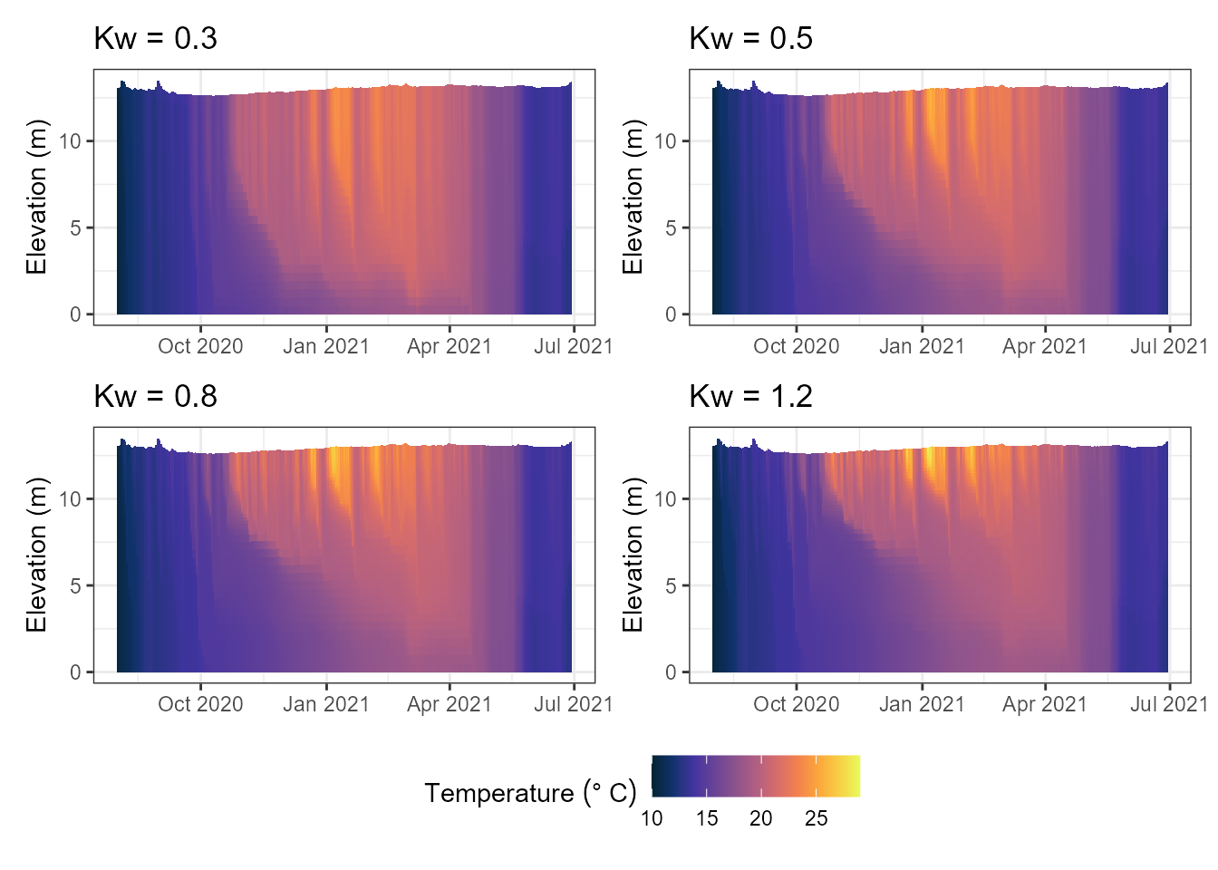

For anything past a handful of candidates – a real sensitivity sweep or a calibration – reach for aemetools instead (aemetools::run_aeme_param()/sa_aeme()/calib_aeme()), which builds on the same idea but works from the full parameter table and the Aeme object, with proper sampling designs and PEST++ integration.

When something goes wrong

By default (safe = TRUE) a failed edit or model run is caught and reported with a message rather than stopping – useful when looping over many candidate scenarios and one bad combination shouldn’t abort the rest:

run_model_test("glm_aed", path_glm, param_overrides = list(lake_depth = -1))
# message: run_model_test error: ... ; returns NULL rather than erroring

Set safe = FALSE while developing a scenario, so a mistake surfaces immediately instead of silently returning NULL.

Next steps

vignette("visualising-output") covers turning out$HYD_temp (or the Aeme object itself) into the plots this kind of comparison is usually for.