Parameter uncertainty with ensembles • AEME

Why parameter uncertainty matters

A single calibrated run gives one trajectory per variable, and it looks far more certain than it is. Many process parameters – light extinction, mixing coefficients, inflow and outflow scaling, the biogeochemical rate constants – are only loosely constrained by the data we have. Several quite different parameter vectors can reproduce the observed temperature profile equally well and then diverge when asked about oxygen, or about a season that was not observed.

Running the model over an ensemble of parameter sets makes that visible. The spread across members is a direct, model-based estimate of how much of the prediction is controlled by what we do not know about the parameters. It is one axis of uncertainty alongside the initial state (see vignette("initial-conditions-and-spin-up")) and the forcing.

This article covers three things:

running an ensemble with run_aeme_ensemble(), here with parameter sets sampled from each parameter’s [min, max] range;
supplying calibrated sets – in particular the posterior from a PEST++ iterative ensemble smoother calibration;
writing the output to Parquet, so a large ensemble can be stored compactly, queried without loading it all, and compared with other ensembles later.

library(AEME)
library(dplyr)
library(ggplot2)

options(AEME.inform = FALSE)

We use the example lake shipped with the package, simulated with GLM-AED. Copy its configuration somewhere writable, load it, and build the model once:

tmpdir <- tempdir()
path <- file.path(tmpdir, "lake")

aeme_file <- system.file("extdata/aeme.rds", package = "AEME")
aeme <- readRDS(aeme_file)

The parameter table

An ensemble needs something to vary. AEME describes calibratable parameters in a long data.frame with one row per parameter: the model and file it lives in, its name, a current value, and the min and max that bound it. The package ships a ready-made table:

data("aeme_parameters", package = "AEME")
param <- aeme_parameters[aeme_parameters$model == "glm_aed", ]
as.data.frame(param[, c("file", "name", "value", "min", "max")])
#>        file                  name value min  max
#> 1  glm3.nml              light/Kw  0.58 0.1 5.52
#> 2  glm3.nml  mixing/coef_mix_conv  0.14 0.1 0.20
#> 3  glm3.nml   mixing/coef_mix_hyp  0.74 0.4 0.80
#> 4  glm3.nml mixing/coef_mix_shear  0.14 0.1 0.20
#> 5  glm3.nml  mixing/coef_mix_turb  0.56 0.2 0.70
#> 6  glm3.nml mixing/coef_wind_stir  0.21 0.2 0.30
#> 7       inf                inflow  1.00 0.5 2.50
#> 8       met            MET_radswd  1.00 0.7 1.30
#> 9       met            MET_wndspd  1.00 0.7 1.30
#> 10      wdr               outflow  1.00 0.5 2.50

The example lake has no parameters attached, so we attach the table to the aeme object with add_param(). The min/max columns are the sampling space, so this is the place to encode what you believe about each parameter. The shipped Kw range (light extinction) runs from 0.1 to 5.5 m^-1, which spans everything from clear alpine water to a bloom; for this lake we narrow it:

param$max[param$name == "light/Kw"] <- 1.5
aeme <- add_param(aeme, param)

Then build the GLM-AED configuration:

aeme <- build_aeme(aeme, model = "glm_aed", path = path, ext_elev = 3)

A sampled ensemble

run_aeme_ensemble() runs a model once per parameter set you give it. For each member it writes the parameters into the model configuration with input_model_parameters() and then calls run_aeme(), and it stores every member’s output on the returned object under output(aeme)$ens_001 ... ens_00k. A member that fails is dropped, with a warning, and the rest are renumbered.

param_sets is either

a list of parameter data.frames, one per member, each with the value column set; or
a single long data.frame with an ensemble id column plus the usual parameter columns.

Each data.frame has the same columns as parameters(aeme); only model, file, name and value are required.

The simplest ensemble draws each parameter independently and uniformly between its min and max. That is a few lines of R, so we write it ourselves:

sample_param_sets <- function(param, n) {
  sets <- lapply(seq_len(n), function(i) {
    p <- param
    p$value <- runif(nrow(p), p$min, p$max)
    p
  })
  setNames(sets, sprintf("m%02d", seq_len(n)))
}

set.seed(42)
param_sets_prior <- sample_param_sets(parameters(aeme), n = 12)
head(param_sets_prior[[1]][, c("name", "value", "min", "max")])
#>                    name     value min max
#> 1              light/Kw 1.3807285 0.1 1.5
#> 2  mixing/coef_mix_conv 0.1937075 0.1 0.2
#> 3   mixing/coef_mix_hyp 0.5144558 0.4 0.8
#> 4 mixing/coef_mix_shear 0.1830448 0.1 0.2
#> 5  mixing/coef_mix_turb 0.5208728 0.2 0.7
#> 6 mixing/coef_wind_stir 0.2519096 0.2 0.3

Then run them:

aeme_prior <- run_aeme_ensemble(aeme, model = "glm_aed", path = path,
                                 param_sets = param_sets_prior)
#> Warning: 4 of 12 ensemble members failed or ended early and were dropped.
#> ℹ Dropped: "m03", "m04", "m10", and "m12".
output(aeme_prior)$n_members
#> [1] 8

Each parameter is sampled independently, so there is no correlation structure between parameters, and every member is a complete model run. Swap in a normal distribution, a Latin hypercube or anything else by changing how value is filled – run_aeme_ensemble() only sees the finished sets.

Members are independent, so they parallelise cleanly. Set parallel = TRUE (and optionally ncore) to run them on several cores, each worker in its own copy of the model directory:

param_sets_prior <- sample_param_sets(parameters(aeme), n = 100)
aeme_prior <- run_aeme_ensemble(aeme, model = "glm_aed", path = path,
                                 param_sets = param_sets_prior,
                                      parallel = TRUE, ncore = 4)

Members that fail

Some combinations of parameters are simply unphysical for a lake – for example an outflow scaling that drains the lake faster than the inflow fills it. GLM does not report that as an error: it exits normally, the water level goes to zero and below, and the rest of the output is NA. run_aeme_ensemble() therefore checks each member’s water level and, by default (drop_incomplete = TRUE), drops any member whose level reaches zero or goes NA, as well as any that error or produce no output. The warning above names the members dropped, and the survivors are renumbered ens_001, ens_002, …

Because the sets were named, the labels of the survivors are kept:

kept <- attr(output(aeme_prior), "realisation")
kept
#> [1] "m01" "m02" "m05" "m06" "m07" "m08" "m09" "m11"
setdiff(names(param_sets_prior), kept)
#> [1] "m03" "m04" "m10" "m12"

Comparing the dropped members’ parameters with the survivors’ shows what went wrong. Here the inflow and outflow scalings are the usual culprits:

bind_rows(param_sets_prior, .id = "member") |>
  filter(name %in% c("inflow", "outflow")) |>
  mutate(status = ifelse(member %in% kept, "kept", "dropped")) |>
  tidyr::pivot_wider(id_cols = c(member, status), names_from = name,
                     values_from = value) |>
  arrange(status, member)
#> # A tibble: 12 × 4
#>    member status  inflow outflow
#>    <chr>  <chr>    <dbl>   <dbl>
#>  1 m03    dropped  1.28    2.17 
#>  2 m04    dropped  0.515   1.72 
#>  3 m10    dropped  1.17    1.74 
#>  4 m12    dropped  0.503   2.16 
#>  5 m01    kept     1.97    1.91 
#>  6 m02    kept     2.46    1.62 
#>  7 m05    kept     2.28    1.74 
#>  8 m06    kept     1.85    1.53 
#>  9 m07    kept     1.04    0.981
#> 10 m08    kept     0.516   0.503
#> 11 m09    kept     0.967   1.11 
#> 12 m11    kept     1.98    0.505

Set drop_incomplete = FALSE to keep every member, NA-padded after the model stopped, if you want to inspect them. A tight parameter range, or a supplied ensemble that has already been through a calibration, is the best way to avoid failures in the first place.

Summarising and plotting

plot_ensemble() shows the central interval of the ensemble as a ribbon, with the lake observations overlaid, for one variable and depth:

plot_ensemble(aeme_prior, model = "glm_aed", var_sim = "HYD_temp", depth = 1,
              conf_int = 0.95)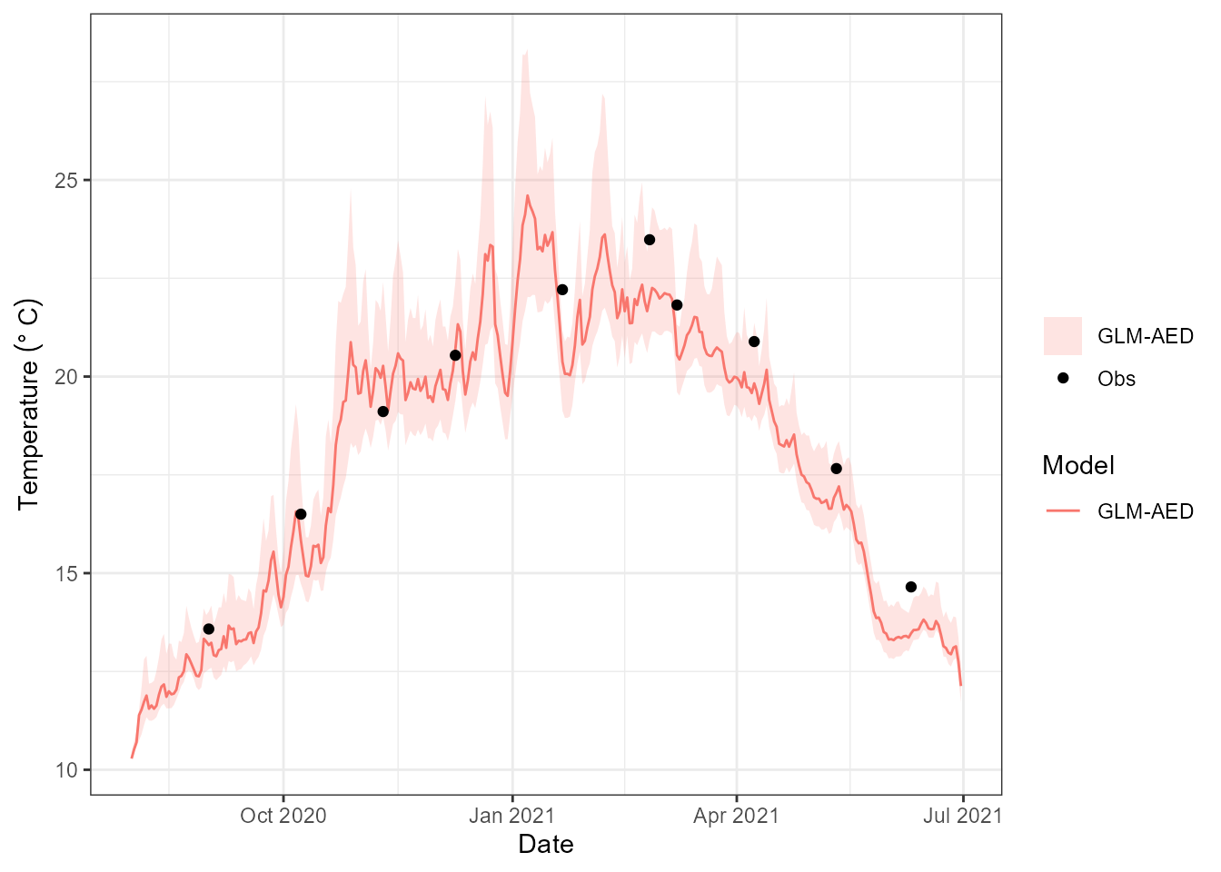

type = "line" draws one line per member instead, which is useful for seeing whether the spread comes from a few outlying members or from the ensemble as a whole:

plot_ensemble(aeme_prior, model = "glm_aed", var_sim = "HYD_temp", depth = 10,
              type = "line")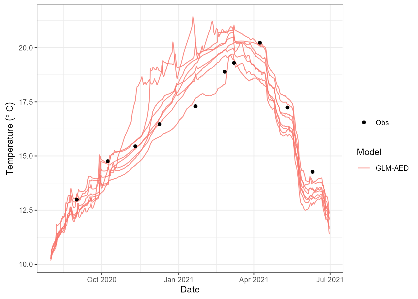

Extracting a variable from every member is the slow part of both plots. If you want several variables or depths, extract once with ensemble_summary() and hand the result to plot_ensemble():

s <- ensemble_summary(aeme_prior, model = "glm_aed",
                      vars_sim = "HYD_temp", depths = c(1, 10))
s
#> <aeme_ensemble_summary>
#>   members  : 8 (kept)
#>   variables: HYD_temp
#>   depths   :  1, 10 (surface-ref)
#>   period   : 2020-08-01 .. 2021-06-30  (668 rows in $stats)
#>   quantiles:  2.5, 25.0, 50.0, 75.0, 97.5 %
#>   obs      : 20 points
head(as.data.frame(s))
#>         Date   Model  var_sim depth n     mean         sd     q2.5      q25
#> 1 2020-08-01 GLM-AED HYD_temp     1 8 10.32730 0.08078228 10.24670 10.27218
#> 2 2020-08-01 GLM-AED HYD_temp    10 8 10.26396 0.06085934 10.18120 10.23822
#> 3 2020-08-02 GLM-AED HYD_temp     1 8 10.56919 0.11266815 10.46019 10.48680
#> 4 2020-08-02 GLM-AED HYD_temp    10 8 10.53059 0.10494376 10.39954 10.46220
#> 5 2020-08-03 GLM-AED HYD_temp     1 8 10.77278 0.16726338 10.58951 10.65813
#> 6 2020-08-03 GLM-AED HYD_temp    10 8 10.63944 0.12301179 10.49408 10.56227
#>        q50      q75    q97.5
#> 1 10.28455 10.39758 10.44355
#> 2 10.24570 10.29950 10.36047
#> 3 10.51405 10.68700 10.72085
#> 4 10.49530 10.62017 10.67714
#> 5 10.70155 10.92507 11.00881
#> 6 10.58610 10.75743 10.80561

Supplying your own parameter sets

Sampling from the bounds answers “what if I only know each parameter lies somewhere in this range?” Often you know more than that. A calibration leaves you with parameter vectors that are already consistent with observations, and you want to propagate those through the model. That needs no new function: the same param_sets argument takes them.

Here we build a small set by hand: twelve members scattered around the current values with a standard deviation of 10 % of each parameter’s range, clipped to the bounds. This stands in for what a calibration would give you:

set.seed(1)
param_sets <- bind_rows(
  lapply(seq_len(12), function(i) {
    p <- parameters(aeme)
    p <- p[p$model == "glm_aed", ]
    p$value <- pmin(pmax(rnorm(nrow(p), p$value, 0.1 * (p$max - p$min)),
                         p$min), p$max)
    p
  }),
  .id = "ensemble"
)
head(param_sets[, c("ensemble", "name", "value", "min", "max")])
#>   ensemble                  name     value min max
#> 1        1              light/Kw 0.4922965 0.1 1.5
#> 2        1  mixing/coef_mix_conv 0.1418364 0.1 0.2
#> 3        1   mixing/coef_mix_hyp 0.7065749 0.4 0.8
#> 4        1 mixing/coef_mix_shear 0.1559528 0.1 0.2
#> 5        1  mixing/coef_mix_turb 0.5764754 0.2 0.7
#> 6        1 mixing/coef_wind_stir 0.2017953 0.2 0.3

aeme_post <- run_aeme_ensemble(aeme, model = "glm_aed", path = path,
                                param_sets = param_sets)
output(aeme_post)$n_members
#> [1] 11

If the ensemble ids are named (as here), the surviving ids are kept on attr(output(aeme_post), "realisation"), so you can map ens_001, ens_002, … back to your own labels after any failed members are removed.

plot_ensemble(aeme_post, model = "glm_aed", var_sim = "HYD_temp", depth = 1)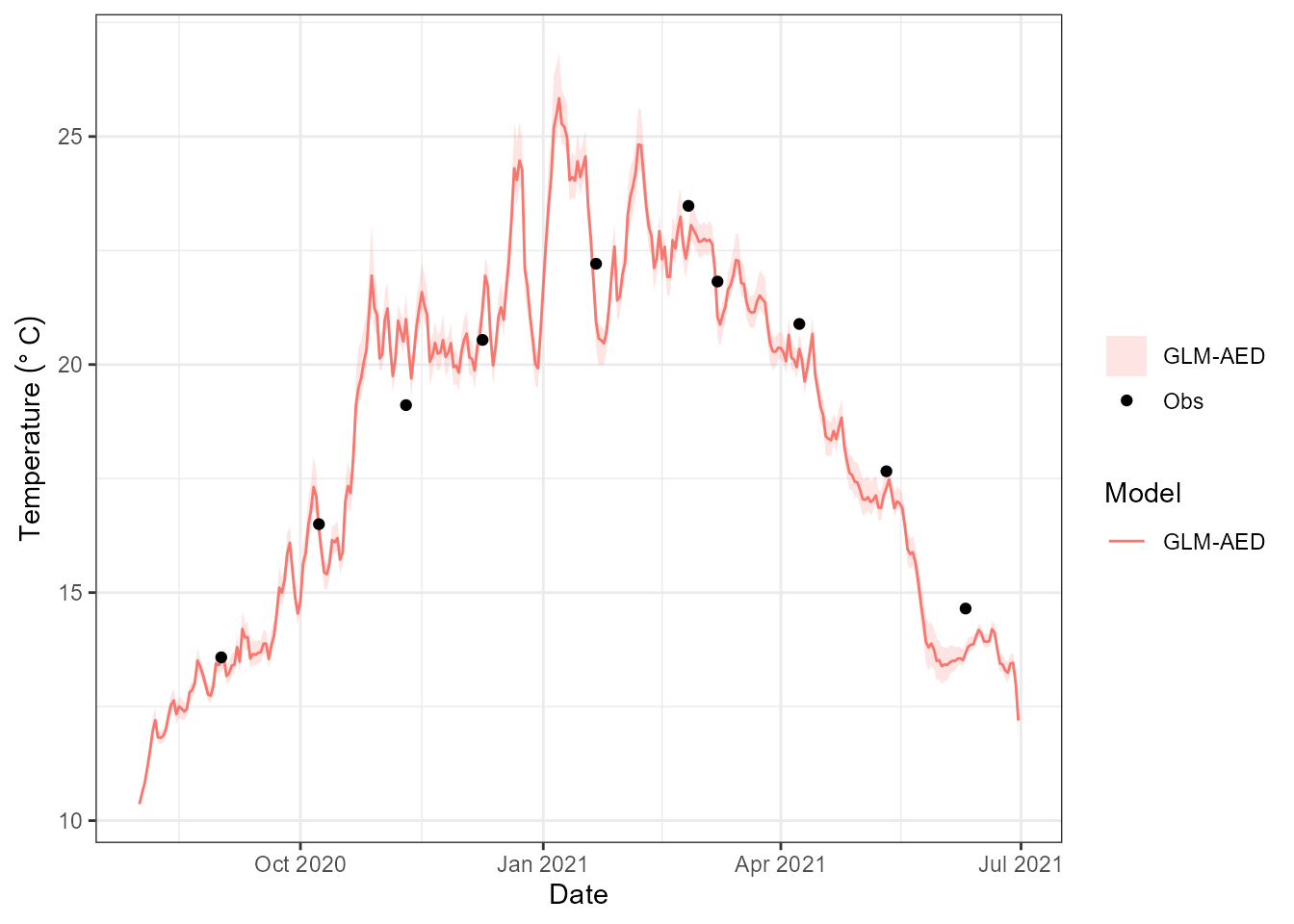

The posterior from a PEST++ calibration

The most useful thing to supply is the posterior ensemble from a pestpp-ies calibration. An iterative ensemble smoother does not return a single “best” parameter set: it returns a whole ensemble of parameter vectors, each of which fits the observations, and the spread among them reflects how well the data constrain each parameter. aemetools::pest_posterior_params() turns that ensemble into a param_sets list that run_aeme_ensemble() can run directly.

# a finished pestpp-ies calibration -- see the aemetools "staged-calibration"
# vignette for how to set one up
calib <- aemetools::read_calib(ctrl = cal_ctrl, sim_id = cal_id)

post <- aemetools::pest_posterior_params(calib)
post

aeme_post <- run_aeme_ensemble(aeme, model = "glm_aed", path = path,
                                param_sets = post, parallel = TRUE)
plot_ensemble(aeme_post, model = "glm_aed", var_sim = "HYD_temp", depth = 1)

Some details worth knowing:

Every set is complete. Parameters that were held fixed during the calibration (frozen in an earlier stage, or with value == min == max) are carried through from the calibration’s parameter metadata, because the smoother only holds the adjustable ones.
iteration = 0 returns the prior ensemble instead, so you can run both and compare the prior and posterior predictive spread: pest_posterior_params(calib, iteration = 0).
n_max keeps only the first few realisations for a quick look at a large ensemble, and include_base = TRUE also keeps the base realisation (the initial parameter values).

The workflow of the whole calibration is described in the aemetools repository.

Writing the output to Parquet

An ensemble is big: every member holds every variable at every layer and every timestep. A 100-member ensemble of a multi-year run is awkward to keep as an .rds – it all has to be loaded to use any of it. AEME can instead write the output to a Parquet store with write_aeme_parquet(). Parquet is a compact, columnar format that R, Python, DuckDB and most data tools read natively, and arrow can query it without reading it all into memory.

pq_prior <- file.path(tmpdir, "parquet_prior")
write_aeme_parquet(aeme_prior, out_root = pq_prior, depths = c(1, 10))

The depths argument says where to summarise depth-resolved variables such as temperature – here 1 m and 10 m below the surface. It is explained under Depth-resolved variables below; without it the summary tier is only really useful for variables with no depth dimension.

(write_aeme_parquet() needs the arrow package.) The store is Hive-partitioned, so each lake and model has its own directory:

list.files(pq_prior, recursive = TRUE)
#> [1] "lakes.parquet"                                               
#> [2] "output_raw/lake_id=LID45819/model=glm_aed/part-0.parquet"    
#> [3] "output_summary/lake_id=LID45819/model=glm_aed/part-0.parquet"

There are two tiers of output per model:

Tier	Contents	Use it for
`output_raw`	Every member’s series: `date`, `ens`, `var_sim`, `depth`, `value`	Drill-down into one lake – spaghetti plots, per-member checks
`output_summary`	Ensemble `mean`, `sd`, `n_ens` and quantiles (`q05`, `q25`, `q50`, `q75`, `q95`) per `date`/`var_sim`/`depth`, with a `depth_ref` column saying what `depth` is measured from	Overview views, many lakes at once, without recomputing the collapse

output_summary is only written when there is more than one member. The quantiles argument sets which quantiles are stored, and compression chooses the Parquet codec: "gzip" (the default) is smallest, "snappy" is fastest to read and write, and "zstd" sits between them.

A one-row-per-lake table, lakes.parquet, records what was exported, including how many ensemble members each lake has:

read_aeme_parquet(pq_prior, what = "lakes")
#>    lake_id    name latitude longitude elevation depth   area      start
#> 1 LID45819 Wainamu -36.8898   174.469     23.64 13.07 152343 2020-08-01
#>         stop  models n_ens
#> 1 2021-06-30 glm_aed     8

Reading it back

read_aeme_parquet() filters by lake_id, model, var_sim and date_range before reading, so asking for one variable never touches the others on disk. For a scalar variable such as lake level the summary tier is all we need, and the ribbon can be drawn without re-running or even loading the model:

lvl <- read_aeme_parquet(pq_prior, what = "output_summary",
                         var_sim = "LKE_lvlwtr")
head(lvl)
#> # A tibble: 6 × 14
#>   date       var_sim  depth depth_ref  mean     sd n_ens   q05   q25   q50   q75
#>   <date>     <chr>    <dbl> <chr>     <dbl>  <dbl> <int> <dbl> <dbl> <dbl> <dbl>
#> 1 2020-08-01 LKE_lvl…    NA NA         13.0 0.0764     8  13.0  13.0  13.0  13.0
#> 2 2020-08-02 LKE_lvl…    NA NA         13.1 0.107      8  13.0  13.0  13.0  13.1
#> 3 2020-08-03 LKE_lvl…    NA NA         13.2 0.170      8  13.0  13.1  13.1  13.2
#> 4 2020-08-04 LKE_lvl…    NA NA         13.8 0.448      8  13.3  13.4  13.8  14.1
#> 5 2020-08-05 LKE_lvl…    NA NA         13.9 0.582      8  13.3  13.4  13.9  14.3
#> 6 2020-08-06 LKE_lvl…    NA NA         13.9 0.704      8  13.2  13.4  13.8  14.4
#> # ℹ 3 more variables: q95 <dbl>, lake_id <chr>, model <chr>

ggplot(lvl, aes(date)) +
  geom_ribbon(aes(ymin = q05, ymax = q95), alpha = 0.25) +
  geom_ribbon(aes(ymin = q25, ymax = q75), alpha = 0.35) +
  geom_line(aes(y = q50)) +
  labs(x = NULL, y = "Water level (m)") +
  theme_bw()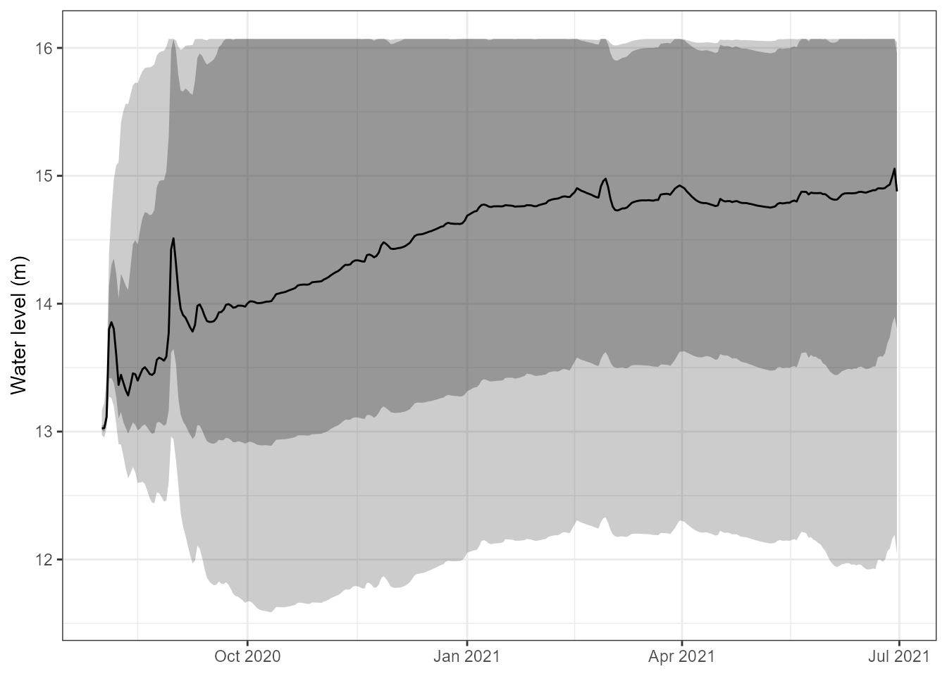

Depth-resolved variables

Variables with a depth dimension need a little more care. AEME interpolates GLM’s own layers onto a standard grid when it loads the output, but that grid is a set of fractions of the water depth scaled to the lake level on each day, not a fixed set of depths. Members whose water level differs – as the inflow and outflow parameters make them – therefore report slightly different depths on the same date (on one day, eight members gave seven different depths for the same grid point, 1.60–1.90 m), and each member’s depths drift as its level moves. Collapsing across members at those depths would leave most groups holding a single member. The raw tier keeps the stored depths as they are, but for the summary tier write_aeme_parquet() takes depths: each member’s profile is interpolated to those depths on every date, and only then are the members collapsed. We asked for 1 m and 10 m when we wrote the store, so every member contributes at both depths:

temp_prior <- read_aeme_parquet(pq_prior, what = "output_summary",
                                var_sim = "HYD_temp")
head(temp_prior[, c("date", "depth", "depth_ref", "mean", "q05", "q50", "q95",
                    "n_ens")])
#> # A tibble: 6 × 8
#>   date       depth depth_ref  mean   q05   q50   q95 n_ens
#>   <date>     <dbl> <chr>     <dbl> <dbl> <dbl> <dbl> <int>
#> 1 2020-08-01     1 surface    10.3  10.3  10.3  10.4     8
#> 2 2020-08-01    10 surface    10.3  10.2  10.2  10.4     8
#> 3 2020-08-02     1 surface    10.6  10.5  10.5  10.7     8
#> 4 2020-08-02    10 surface    10.5  10.4  10.5  10.7     8
#> 5 2020-08-03     1 surface    10.8  10.6  10.7  11.0     8
#> 6 2020-08-03    10 surface    10.6  10.5  10.6  10.8     8
table(temp_prior$depth, temp_prior$n_ens)
#>     
#>        8
#>   1  334
#>   10 334

n_ens counts the members that have a value. A depth that falls outside a member’s water column on a date – deeper than that member’s lake, or above its surface – is left out for that member rather than guessed at, so n_ens drops below the ensemble size there.

depth_ref chooses what depths is measured from. The default, "surface", is metres below the water surface. With "bottom" it is metres above the lake bed, so depths = 1 is the water 1 m above the bottom. That is a different height below the surface on every date and for every member, because the water level differs, so it is worked out from each member’s own level (LKE_lvlwtr):

pq_bottom <- file.path(tmpdir, "parquet_bottom")
write_aeme_parquet(aeme_prior, out_root = pq_bottom, depths = 1,
                   depth_ref = "bottom")

bottom <- read_aeme_parquet(pq_bottom, what = "output_summary",
                            var_sim = "HYD_temp")
head(bottom[, c("date", "depth", "depth_ref", "mean", "q50", "n_ens")])
#> # A tibble: 6 × 6
#>   date       depth depth_ref  mean   q50 n_ens
#>   <date>     <dbl> <chr>     <dbl> <dbl> <int>
#> 1 2020-08-01     1 bottom     10.3  10.2     8
#> 2 2020-08-02     1 bottom     10.5  10.5     8
#> 3 2020-08-03     1 bottom     10.6  10.6     8
#> 4 2020-08-04     1 bottom     10.7  10.7     8
#> 5 2020-08-05     1 bottom     10.8  10.8     8
#> 6 2020-08-06     1 bottom     10.9  10.9     8

The raw tier is unchanged by depths and depth_ref: it always holds the stored depths, in metres below the surface.

For a big store, push the filter into the Parquet scan with collect = FALSE, which returns a lazy arrow query. Further dplyr verbs are applied before any data is pulled into R:

ds <- read_aeme_parquet(pq_prior, what = "output_raw", var_sim = "HYD_temp",
                        date_range = c("2021-01-01", "2021-01-31"),
                        collect = FALSE)
class(ds)[1]
#> [1] "arrow_dplyr_query"

ds |>
  filter(!is.na(value)) |>
  group_by(ens) |>
  summarise(mean_temp = mean(value), n = n()) |>
  collect()
#> # A tibble: 8 × 3
#>     ens mean_temp     n
#>   <int>     <dbl> <int>
#> 1     1      19.3  1333
#> 2     2      19.6  1457
#> 3     3      20.6  1457
#> 4     4      20.2  1457
#> 5     5      21.2  1333
#> 6     6      20.4  1333
#> 7     7      20.2  1302
#> 8     8      20.6  1457

Comparing ensembles

Because a store is just files, keeping several ensembles side by side is straightforward. One thing to watch: the partitions are keyed by lake_id and model, so re-exporting the same lake to the same out_root replaces its data. Write each ensemble you want to keep to its own out_root.

Here we export the narrower, supplied ensemble to a second store and compare it with the one sampled from the full parameter ranges:

pq_post <- file.path(tmpdir, "parquet_post")
write_aeme_parquet(aeme_post, out_root = pq_post, depths = c(1, 10))

temp_post <- read_aeme_parquet(pq_post, what = "output_summary",
                               var_sim = "HYD_temp")

both <- bind_rows(prior = temp_prior, narrowed = temp_post, .id = "ensemble")

ggplot(both, aes(date, fill = ensemble, colour = ensemble)) +
  geom_ribbon(aes(ymin = q05, ymax = q95), alpha = 0.25, colour = NA) +
  geom_line(aes(y = q50)) +
  facet_wrap(~ paste(depth, "m"), ncol = 1, scales = "free_y") +
  labs(x = NULL, y = "Temperature (°C)", fill = NULL, colour = NULL) +
  theme_bw()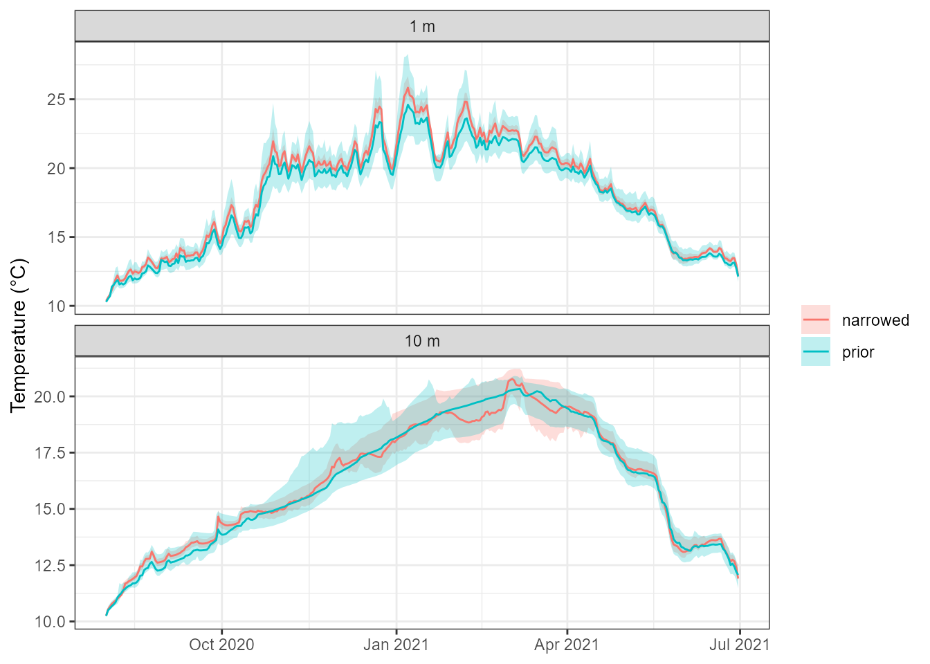

The width of each band is the output uncertainty attributable to the parameters. Two cautions when reading this particular plot. The narrowed ensemble is only a tighter scatter around the current values, not a calibration, so it need not be narrower everywhere. And the wide ensemble lost the members that drained the lake (see Members that fail), so its band is built from fewer members than were sampled.

With a real calibration the comparison is the point: store the iteration = 0 prior and the final posterior of a PEST++ run the same way. Where the posterior is clearly narrower, the data have constrained what the model can do.

Size on disk for the twelve sampled members, with both tiers and every output variable written:

files <- list.files(pq_prior, recursive = TRUE, full.names = TRUE)
round(sum(file.size(files)) / 1e6, 1)  # MB, both tiers
#> [1] 5.8

Because every lake is just another lake_id= partition, the same out_root can hold many lakes, and read_aeme_parquet() (or DuckDB, Python, …) can query them all at once.

Practical guidance

Question	Guidance
How many members?	Cost is one full model run per member. Start with 10–20 to check the setup and the ranges, then increase until the quantiles you care about stop moving. Use `parallel = TRUE` for anything large.
What should the ranges be?	`min` and `max` are your prior. Overly wide ranges produce unphysical members (see Members that fail), which are dropped, so you pay for runs you cannot use; narrow them to what is physically defensible for the lake.
Sampled or supplied?	Sample from the bounds for exploration and as a prior. Supply parameter sets (e.g. a PEST++ posterior) when you want to propagate calibrated uncertainty.
Which output to keep?	`output_raw` keeps everything and lets you recompute anything later; `output_summary` is smaller and quicker for overviews, but its depths are scaled to each member’s water level and so do not line up across members – interpolate depth-resolved variables to fixed depths from the raw tier.
What does the spread mean?	Only parameter uncertainty. Forcing, initial conditions and structural error are not represented; for the initial state see `vignette("initial-conditions-and-spin-up")`.