
Lake Rotoehu Water Balance and Evaporation
Source:vignettes/articles/rotoehu-water-balance.Rmd
rotoehu-water-balance.RmdIntroduction
This article demonstrates how to work with Lake Rotoehu (ID: 40188) to:
- Set up an AEME model using data from the
aemetoolspackage - Understand the three water balance approaches and when to use each
- Understand how lake surface temperature is estimated (and the role of observations)
- Learn how evaporation is estimated from bulk aerodynamic theory
- Extract and visualise evaporation output
Lake Rotoehu is a small, shallow lake in the Rotorua region of New Zealand’s North Island (~8 km² surface area, ~13 m maximum depth). It is eutrophic, thermally stratifies in summer, and has no permanent gauged inflow — making a water-balance approach particularly useful for constraining its hydrology.
Load Lake Rotoehu data
The aemetools package provides access to pre-configured
AEME objects for New Zealand lakes via the Limnotrack API. Use the
lake’s numeric ID to retrieve it:
aeme <- aemetools::get_aeme(id = 40188)View Aeme object:
aeme
#>
#> ── AEME not yet built ──────────────────────────────────────────────────────────
#>
#> ── Lake ──
#>
#> Rotoehu (ID: LID40188)
#> • Lat: -38.01; Lon: 176.53
#> • Elev: 302.97m; Depth: 22.7m; Area: 7965248 m2
#>
#> ── Time ──
#>
#> • Start: 2010-06-01 00:00:00; Stop: 2023-06-30 00:00:00; Time step: 3600 s;
#> Output step: 86400 s
#> • Timezone: UTC (timestamps stored UTC)
#> • Spin up (days): GLM: 365; GOTM: 365; DYRESM: 365; Simstrat: 365
#>
#> ── Configuration ──
#>
#> • Model: glm_aed and gotm_wet
#> • Path: Not set
#> • Model controls: Present
#> • Use biogeochemical model:
#> ┌ Model Configuration ─────────────────────────────────────────┐
#> │ Model Physical Biogeochemical │
#> │ --- │
#> │ DY-CD Absent Absent │
#> │ GLM-AED Present Absent │
#> │ GOTM-WET Present Absent │
#> │ SIMSTRAT-AED2 Absent Absent │
#> │ SIMSTRAT-AED Absent Absent │
#> └──────────────────────────────────────────────────────────────┘
#>
#> ── Observations ──
#>
#> • Lake: Present; Level: Absent
#>
#> ── Input ──
#>
#> • Initial profile: Present; Initial depth: 22.698m
#> • Hypsograph: Present (n=64)
#> • Meteo: Present; Use longwave: TRUE; Kw: 0.586206896551724
#>
#> ── Inflows ──
#>
#> • Number of inflows: 3; Names: NZS4079511, NZS4081174, lumped
#> • Scaling factors: DY-CD: 1; GLM-AED: 1; GOTM-WET: 1; Simstrat-AED2: 1
#>
#> ── Outflows ──
#>
#> • Number of outflows: 1; Names: wbal; Elevations: -1
#> • Scaling factors: DY-CD: 1; GLM-AED: 1; GOTM-WET: 1; Simstrat-AED2: 1
#>
#> ── Water Balance ──
#>
#> • Method: 2; Use: obs
#> • Modelled: Absent; Water balance: Present
#>
#> ── Parameters ──
#>
#> • Number of parameters: 0
#>
#> ── Output ──
#>
#> • DY-CD: 1
#> • GLM-AED: 1
#> • GOTM-WET: 1
#> • SIMSTRAT-AED2: 0
#> • SIMSTRAT-AED: 0
#> • Variables: 64
#> Water temperature, Thermocline depth, Dissolved oxygen, Total chlorophyll a,
#> Total nitrogen, Total phosphorus, Water level, LKE_V, Change in volume, Surface
#> area, ... and 54 moreView and update the hypsograph
The hypsograph encodes the depth–area relationship and is central to all volume and evaporation calculations. Let’s inspect what was loaded:
hyps <- get_hypsograph(aeme)
orig_hyps <- hyps |>
dplyr::filter(depth <= 0)
ggplot(orig_hyps, aes(x = area, y = depth)) +
geom_line(colour = "#0065a9", linewidth = 0.8) +
labs(x = "Area (m²)", y = "Depth (m)",
title = "Original Hypsograph for Lake Rotoehu") +
theme_bw()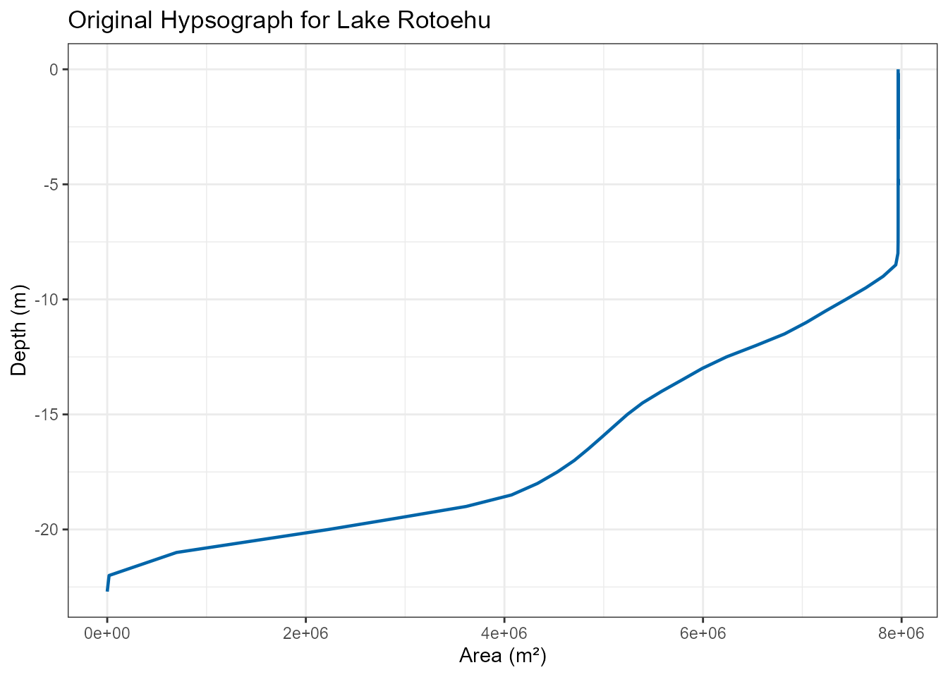
This does not look right — the max depth is too deep and there is about 8m from the surface to the first contour. We can improve this by building a new hypsograph from bathymetric contours available on the Limnotrack API:
# Lake Rotoehy lake id is 40188
shoreline <- aemetools::get_lake_shape(id = 40188) # lake shoreline shapefile
# Get lake depth contours
contours <- ltapi::lt_fetch(
"lake_contours",
filter = ltapi::lt_filter(lernzmp_id == "LID40188")
) |>
dplyr::mutate(depth = depth_m)