Introduction
The Lake Ecosystem Research New Zealand Model Platform (LERNZmp) is a web platform that provides a user-friendly interface to the lake ecosystem model output for New Zealand lakes. The platform is designed to provide a simple way to explore the model output across multiple lakes and also to compare the model results with observed data.
The platform is located here: LERNZmp. Select and load a lake model output on the “Overview” tab. The model output can be downloaded in the “Download Models” tab. This downloads a “.zip” folder containing the model output for the selected lake(s) as “.rds” files and a lake metadata file “LERNZmp_lake_metadata.csv”.
Using LERNZmp output with AEME
Once you have downloaded the LERNZmp model output and unzipped the folder, you should have a similar file structure to the following:
list.files("lernzmp")
#> [1] "LERNZmp_lake_metadata.csv" "LID11133.rds"
#> [3] "LID40102.rds"              "LID45819.rds"
LERNZmp metadata
The metadata file contains information about the all the lakes in the LERNZmp platform. This includes the lake ID, name surface area (ha), region, geomorphic type, depth, depth measurement (measured or predicted), data (no data/minimal data/limited and irregular/periodic but sparse/seasonal but detailed) and lernzmp file name.
metadata <- read.csv("lernzmp/LERNZmp_lake_metadata.csv")
head(metadata)
#>        ID            Name   Area     Region Geomorphic.type Depth
#> 1   LID 1           Onoke 622.34 Wellington       Shoreline  8.72
#> 2   LID 3 Kohangapiripiri  10.82 Wellington       Shoreline 14.43
#> 3   LID 4     Kohangatera  21.31 Wellington       Shoreline 14.80
#> 4 LID 119         LID 119  41.87 Wellington        Riverine  3.55
#> 5 LID 195         Nganoke   3.10 Wellington        Riverine  3.74
#> 6 LID 229          Pounui  45.95 Wellington        Tectonic    NA
#>   Depth.measurement         Data aeme_file
#> 1          Measured Minimal Data      LID1
#> 2         Predicted      No data      LID3
#> 3         Predicted      No data      LID4
#> 4         Predicted      No data    LID119
#> 5         Predicted      No data    LID195
#> 6         Predicted      No data    LID229
RDS files
RDS files are binary files that store R objects, such as data sets,
and are a native format for R. RDS files preserve data types and classes
and are generally smaller than their text file counterparts. The AEME
objects are an S4 object of the class Aeme. This object
class an store model configuration, inputs and outputs and allows for
the easy transfer of a lake model setup.
The lakes included in this example have ID’s LID11133 and LID40102. We will filter the metadata to examine these two lakes.
metadata <- metadata |>
  dplyr::filter(aeme_file %in% c("LID11133", "LID40102"))
metadata
#>          ID    Name    Area        Region Geomorphic.type Depth
#> 1 LID 11133 Rotorua 8060.23 Bay of Plenty        Volcanic 45.27
#> 2 LID 40102  Rotoma 1113.68 Bay of Plenty        Volcanic 89.13
#>   Depth.measurement                  Data aeme_file
#> 1          Measured Seasonal but Detailed  LID11133
#> 2          Measured Seasonal but Detailed  LID40102
These are lakes Rotorua (LID11133) and Rotoma (LID40102), respectively.
Build AEME models
We will now build AEME models for these two lakes using the LERNZmp model output. We will first load the AEME object from the “.rds” files.
The Aeme object contains the lake metadata, model
output, and model controls. More details can be found
vignette("intro-aeme"). It is an S4 object of the class
Aeme.
First, make sure to install the AEME package.
# install.packages("remotes")
remotes::install_github("limnotrack/AEME")
Once installed, load the AEME package.
library(AEME)
#>
#> Attaching package: 'AEME'
#> The following object is masked from 'package:stats':
#>
#>     time
Now, we will load the AEME object for Lake Rotorua (LID11133).
It can be printed to the console to see the contents of the object.
aeme
#> Warning: ! Lake observations use the legacy depth_from / depth_to columns.
#> ℹ These have been collapsed to a single depth column (interval midpoint).
#>   Update your data to the current schema ("Date", "var_aeme", "depth", and
#>   "value"); depth_to and sd are optional.
#> This warning is displayed once per session.
#> Warning: ! This <Aeme> object has no recorded AEME package version.
#> ℹ It was likely built with an older version of AEME (<0.4.0), or has never been
#>   built with `build_aeme()`. Consider rebuilding with `build_aeme()` to keep it
#>   in sync with the installed package (0.4.0).
#> This warning is displayed once per session.
#>
#> ── AEME not yet built ──────────────────────────────────────────────────────────
#>
#> ── Lake ──
#>
#> Rotorua (ID: LID11133)
#> • Lat: -38.09; Lon: 176.27
#> • Elev: 284.88m; Depth: 48.15m; Area: 80659960 m2
#>
#> ── Time ──
#>
#> • Start: 2013-07-01 00:00:00; Stop: 2023-06-30 00:00:00; Time step: 3600 s;
#>   Output step: s
#> • Timezone: UTC (timestamps stored UTC)
#> • Spin up (days): GLM: 1095; GOTM: 1095; DYRESM: 1095; Simstrat: 2
#>
#> ── Configuration ──
#>
#> • Model: glm_aed and gotm_wet
#> • Path: Not set
#> • Model controls: Present
#> • Use biogeochemical model:
#> ┌ Model Configuration ─────────────────────────────────────────┐
#> │       Model              Physical         Biogeochemical     │
#> │ ---                                                          │
#> │       DY-CD               Absent              Absent         │
#> │      GLM-AED             Present              Absent         │
#> │      GOTM-WET            Present              Absent         │
#> │   SIMSTRAT-AED2           Absent              Absent         │
#> │    SIMSTRAT-AED           Absent              Absent         │
#> └──────────────────────────────────────────────────────────────┘
#>
#> ── Observations ──
#>
#> • Lake: Present; Level: Absent
#>
#> ── Input ──
#>
#> • Initial profile: Present; Initial depth: 48.148m
#> • Hypsograph: Present (n=95)
#> • Meteo: Present; Use longwave: TRUE; Kw: 0.566666666666667
#>
#> ── Inflows ──
#>
#> • Number of inflows: 7; Names: NZS4081641, NZS4083363, NZS4084132, NZS4086165,
#>   NZS4084816, lumped, precip
#> • Scaling factors: DY-CD: 1; GLM-AED: 1; GOTM-WET: 1; Simstrat-AED2: 1
#>
#> ── Outflows ──
#>
#> • Number of outflows: 1; Names: wbal; Elevations: -1
#> • Scaling factors: DY-CD: 1; GLM-AED: 1; GOTM-WET: 1; Simstrat-AED2: 1
#>
#> ── Water Balance ──
#>
#> • Method: 2; Use: obs
#> • Modelled: Absent; Water balance: Present
#>
#> ── Parameters ──
#>
#> • Number of parameters: 18
#>
#> ── Output ──
#>
#> • DY-CD: 1
#> • GLM-AED: 1
#> • GOTM-WET: 1
#> • SIMSTRAT-AED2: 0
#> • SIMSTRAT-AED: 0
#> • Variables: 64
#> Water temperature, Thermocline depth, Dissolved oxygen, Total chlorophyll a,
#> Total nitrogen, Total phosphorus, Water level, LKE_V, Change in volume, Surface
#> area, ... and 54 more
This allows for quick inspection of all the different slots within
the Aeme object. The lake section has the lake metadata,
the time section has the start, stop and spin-up dates, the
configuration section has the model configuration which allows for the
building of the AEME models locally.
model <- c("glm_aed", "gotm_wet") # models to build
path <- "aeme" # directory in which the model configuration will be built

aeme <- build_aeme(aeme = aeme, model = model, path = path,
                   use_bgc = TRUE)
#> ✔ `MET_pprain`: converted from m/day to mm/day.
#> Warning: GLM ignores the AirPres met column in daily mode and uses the default 1013.25 hPa instead.
#> This warning is displayed once per session.
Run AEME models
We will now run the AEME models for the two lakes. This will run the
models with the configurations built in the path directory.
The parallel argument is set to TRUE to run
the models in parallel which can speed up the process.
aeme <- run_aeme(aeme = aeme, model = model, path = path, parallel = TRUE)
aeme
#>
#> ── AEME v0.4.0 ─────────────────────────────────────────────────────────────────
#>
#> ── Lake ──
#>
#> Rotorua (ID: LID11133)
#> • Lat: -38.09; Lon: 176.27
#> • Elev: 284.88m; Depth: 48.15m; Area: 80659960 m2
#>
#> ── Time ──
#>
#> • Start: 2013-07-01 00:00:00; Stop: 2023-06-30 00:00:00; Time step: 3600 s;
#>   Output step: s
#> • Timezone: UTC (timestamps stored UTC)
#> • Spin up (days): GLM: 1095; GOTM: 1095; DYRESM: 1095; Simstrat: 2
#>
#> ── Configuration ──
#>
#> • Model: glm_aed and gotm_wet
#> • Path: D:\a\AEME\AEME\vignettes\articles\aeme
#> • Model controls: Present
#> • Use biogeochemical model: Yes
#> ┌ Model Configuration ─────────────────────────────────────────┐
#> │       Model              Physical         Biogeochemical     │
#> │ ---                                                          │
#> │       DY-CD               Absent              Absent         │
#> │      GLM-AED             Present             Present         │
#> │      GOTM-WET            Present             Present         │
#> │   SIMSTRAT-AED2           Absent              Absent         │
#> │    SIMSTRAT-AED           Absent              Absent         │
#> └──────────────────────────────────────────────────────────────┘
#>
#> ── Observations ──
#>
#> • Lake: Present; Level: Absent
#>
#> ── Input ──
#>
#> • Initial profile: Present; Initial depth: 48.148m
#> • Hypsograph: Present (n=95)
#> • Meteo: Present; Use longwave: TRUE; Kw: 0.566666666666667
#>
#> ── Inflows ──
#>
#> • Number of inflows: 7; Names: NZS4081641, NZS4083363, NZS4084132, NZS4086165,
#>   NZS4084816, lumped, precip
#> • Scaling factors: DY-CD: 1; GLM-AED: 1; GOTM-WET: 1; Simstrat-AED2: 1
#>
#> ── Outflows ──
#>
#> • Number of outflows: 1; Names: wbal; Elevations: -1, -1
#> • Scaling factors: DY-CD: 1; GLM-AED: 1; GOTM-WET: 1; Simstrat-AED2: 1
#>
#> ── Water Balance ──
#>
#> • Method: 2; Use: obs
#> • Modelled: Absent; Water balance: Present
#>
#> ── Parameters ──
#>
#> • Number of parameters: 18
#>
#> ── Output ──
#>
#> • DY-CD: 0
#> • GLM-AED: 1
#> • GOTM-WET: 1
#> • SIMSTRAT-AED2: 0
#> • SIMSTRAT-AED: 0
#> • Variables: 453
#> Water temperature, Dissolved oxygen, Total chlorophyll a, Total nitrogen, Total
#> phosphorus, Water level, Evaporative heat flux, Sensible heat flux, Longwave
#> radiation, Shortwave radiation, ... and 443 more
In the “Output” section of the Aeme object, the “Number
of ensembles” is set to 1 indicating that there is now output for each
model in the Aeme object.
plot_output(aeme = aeme, model = model, var_sim = "HYD_temp")
#> Warning: Removed 336 rows containing missing values or values outside the scale range
#> (`geom_col()`).
#> Warning: Removed 1482 rows containing missing values or values outside the scale range
#> (`geom_point()`).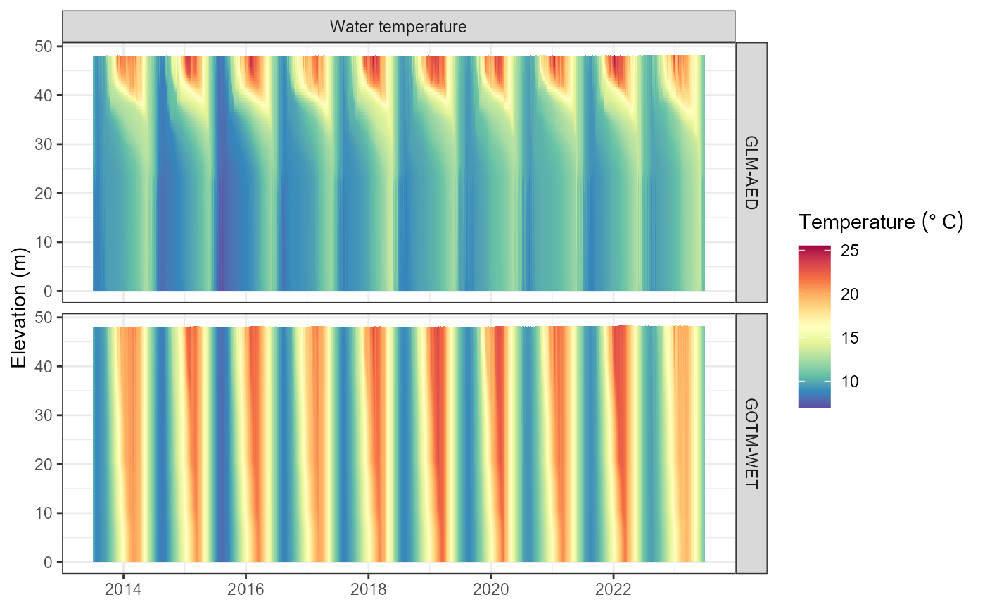
plot_output(aeme = aeme, model = model, var_sim = "CHM_oxy")
#> Warning: Removed 336 rows containing missing values or values outside the scale range
#> (`geom_col()`).
#> Warning: Removed 1586 rows containing missing values or values outside the scale range
#> (`geom_point()`).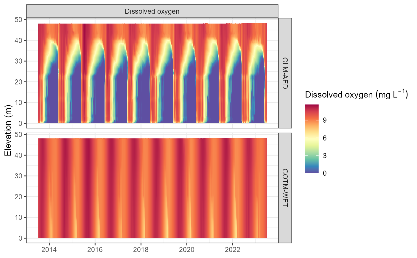
Access AEME input data
The Aeme object contains the input data for the models.
This includes the lake metadata, model controls, and model
configuration. The input slot contains the initial profile
(“init_profile”), initial depth (“init_depth”), hypograph (“hypograph”),
meteorological data (“meteo”), switch for using longwave radiation
(“use_lw”) and light extinction coefficient (“Kw”) for the models.
inp <- input(aeme)
names(inp)
#> [1] "init_profile" "init_depth"   "hypsograph"   "meteo"        "use_lw"
#> [6] "Kw"
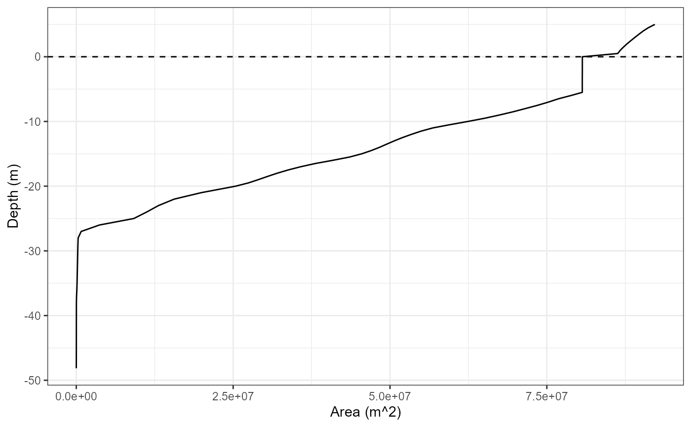
Hypsograph data
hyps <- inp$hypsograph
head(hyps)
#>     elev     area depth
#> 1 289.88 92216772   5.0
#> 2 289.38 91198888   4.5
#> 3 288.88 90383984   4.0
#> 4 288.38 89698688   3.5
#> 5 287.88 89045360   3.0
#> 6 287.38 88405268   2.5
library(ggplot2)
ggplot(hyps, aes(x = area, y = depth)) +
  geom_hline(yintercept = 0, linetype = "dashed") +
  geom_line() +
  labs(y = "Depth (m)", x = "Area (m^2)") +
  theme_bw()