Reservoir Simulation with Multiple Outlets • AEME

Introduction

Reservoirs differ from natural lakes in several ways that are important for hydrodynamic modelling:

Regulated water levels – reservoir levels are managed through controlled releases rather than a natural outlet or seepage.
Multiple outlets at different depths – a single reservoir can have:
- A surface spillway that only activates when the reservoir is near full capacity.
- A penstock or bottom outlet for daily operational releases.
- A mid-level selective withdrawal outlet for water quality management (e.g. to avoid releasing cold, anoxic hypolimnetic water).
Thermal stratification management – withdrawals from different depth layers affect the downstream temperature and water quality.

AEME supports all three major 1-D hydrodynamic models (DYRESM-CAEDYM, GLM-AED, GOTM-WET) with multiple outlets at arbitrary elevations. This vignette walks through setting up a reservoir ensemble model with two outlets at different levels: a regulated penstock at depth and a surface spillway.

Setup

library(AEME)
library(ggplot2)
library(dplyr)

Reservoir data

We will use a fictional reservoir, Reservoir, located in the North Island of New Zealand. The reservoir has a full supply level of 150 m above sea level and a maximum depth of 25 m.

lat   <- -37.80
lon   <- 176.00
elev  <- 150   # full supply level (m a.s.l.)
depth <- 25    # maximum depth (m)
area  <- 1.2e6 # surface area at full supply level (m²)

reservoir <- list(
  name      = "Reservoir",
  id        = "res001",
  latitude  = lat,
  longitude = lon,
  elevation = elev,
  depth     = depth,
  area      = area
)

Simulation period

time <- list(
  start = "2020-08-01 00:00:00",
  stop  = "2021-06-30 00:00:00"
)

Meteorological data

Meteorological data bundled with the AEME package (originally from Lake Wainamu, North Island) is reused here to drive the reservoir simulation.

meteo_file <- system.file("extdata/lake/data/meteo.csv", package = "AEME")
met <- read.csv(meteo_file) |>
  mutate(Date = as.Date(Date))

head(met[, 1:5])
#>         Date MET_tmpair MET_tmpdew MET_wnduvu MET_wnduvv
#> 1 2019-01-01    19.5260    16.9129    3.19505    4.21590
#> 2 2019-01-02    19.5024    15.7136    4.59457    2.62703
#> 3 2019-01-03    20.1359    18.0478    6.17768    3.99858
#> 4 2019-01-04    19.1298    15.2155    2.56012    5.66473
#> 5 2019-01-05    19.1868    15.3679    3.77683    2.75966
#> 6 2019-01-06    20.2102    16.6466    4.83125    3.06035

Hypsograph

The hypsograph describes the relationship between elevation and surface area (and thus volume). Constructed reservoirs typically have a more prismatic (box-like) shape compared to natural lakes. This is reflected by a higher volume_development parameter (values > 1.5 give a convex, cylindrical shape; a value of 3 corresponds to a perfect cylinder).

hypsograph <- generate_hypsograph(
  max_depth          = depth,
  surface_area       = area,
  volume_development = 2.5,   # more prismatic than a natural lake
  elev               = elev,
  ext_elev           = 2      # extend 2 m above full supply level
)

head(hypsograph)
#>    elev depth    area
#> 1 152.0   2.0 1391324
#> 2 150.0   0.0 1200000
#> 3 149.8  -0.2 1176144
#> 4 149.6  -0.4 1152574
#> 5 149.4  -0.6 1129291
#> 6 149.2  -0.8 1106292

ggplot(hypsograph, aes(x = area / 1e6, y = elev)) +
  geom_line(linewidth = 1, colour = "#0065a9") +
  geom_point(size = 1.5, colour = "#0065a9") +
  labs(
    x     = expression("Area (km"^2 * ")"),
    y     = "Elevation (m a.s.l.)",
    title = "Reservoir – hypsograph"
  ) +
  theme_bw()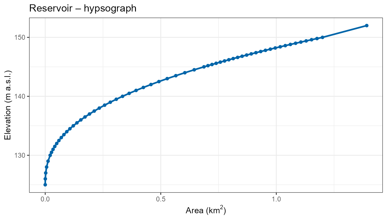

Inflow data

We create a synthetic seasonal inflow time series typical of a New Zealand catchment, with higher flows in winter (June–August) and lower flows in summer. The inflow data frame must contain at minimum Date and HYD_flow (m³ day⁻¹). Temperature (HYD_temp, °C) and salinity (CHM_salt, PSU) columns are recommended.

set.seed(42)
sim_dates <- seq(as.Date("2020-01-01"), as.Date("2021-12-31"), by = "day")
doy       <- as.integer(format(sim_dates, "%j"))

# Seasonal signal: peak winter flow ~day 200 (NZ Southern Hemisphere winter)
inflow_flow <- pmax(5000,
  80000 + 60000 * cos(2 * pi * (doy - 200) / 365) +
    rnorm(length(sim_dates), mean = 0, sd = 8000))

# River temperature: coolest in winter, warmest in summer
inflow_temp <- pmax(4, 15 - 8 * cos(2 * pi * (doy - 15) / 365))

inflow_data <- data.frame(
  Date     = sim_dates,
  HYD_flow = inflow_flow,
  HYD_temp = inflow_temp,
  CHM_salt = 0
)

head(inflow_data[, 1:3])
#>         Date HYD_flow HYD_temp
#> 1 2020-01-01 33371.71 7.231200
#> 2 2020-01-02 17605.56 7.199484
#> 3 2020-01-03 24764.44 7.170079
#> 4 2020-01-04 26675.80 7.142995
#> 5 2020-01-05 24617.84 7.118239
#> 6 2020-01-06 20322.85 7.095819

Multiple outlet data

The key feature demonstrated in this vignette is the configuration of two outlets at different elevations:

Outlet	Elevation	Description
Penstock	130 m	Regulated bottom release; 20 m below full supply level
Spillway	-1 (surface)	Uncontrolled overflow at the water surface

# Penstock: regulated base flow with small seasonal variation
penstock_flow <- pmax(0,
  60000 + 15000 * sin(2 * pi * (doy - 100) / 365) +
    rnorm(length(sim_dates), mean = 0, sd = 4000))

# Spillway: only active during the high-inflow winter period
spillway_flow <- pmax(0,
  25000 * cos(2 * pi * (doy - 200) / 365) +
    rnorm(length(sim_dates), mean = 0, sd = 5000))

penstock_data <- data.frame(
  Date     = sim_dates,
  HYD_flow = penstock_flow
)

spillway_data <- data.frame(
  Date     = sim_dates,
  HYD_flow = spillway_flow
)

Visualise the inflow and both outflows over the simulation period:

flows <- bind_rows(
  mutate(inflow_data[, c("Date", "HYD_flow")], stream = "Inflow"),
  mutate(penstock_data, stream = "Penstock (130 m)"),
  mutate(spillway_data, stream = "Spillway (surface)")
) |>
  filter(Date >= as.Date("2020-08-01"),
         Date <= as.Date("2021-06-30"))

ggplot(flows, aes(x = Date, y = HYD_flow / 1e3, colour = stream)) +
  geom_line(linewidth = 0.8) +
  scale_colour_manual(
    values = c("Inflow"             = "#0065a9",
               "Penstock (130 m)"   = "#d73027",
               "Spillway (surface)" = "#4dac26"),
    name = NULL
  ) +
  labs(
    x     = "Date",
    y     = expression("Flow (×10"^3 * " m"^3 * " day"^{-1} * ")"),
    title = "Simulated inflow and outflow discharges"
  ) +
  theme_bw() +
  theme(legend.position = "bottom")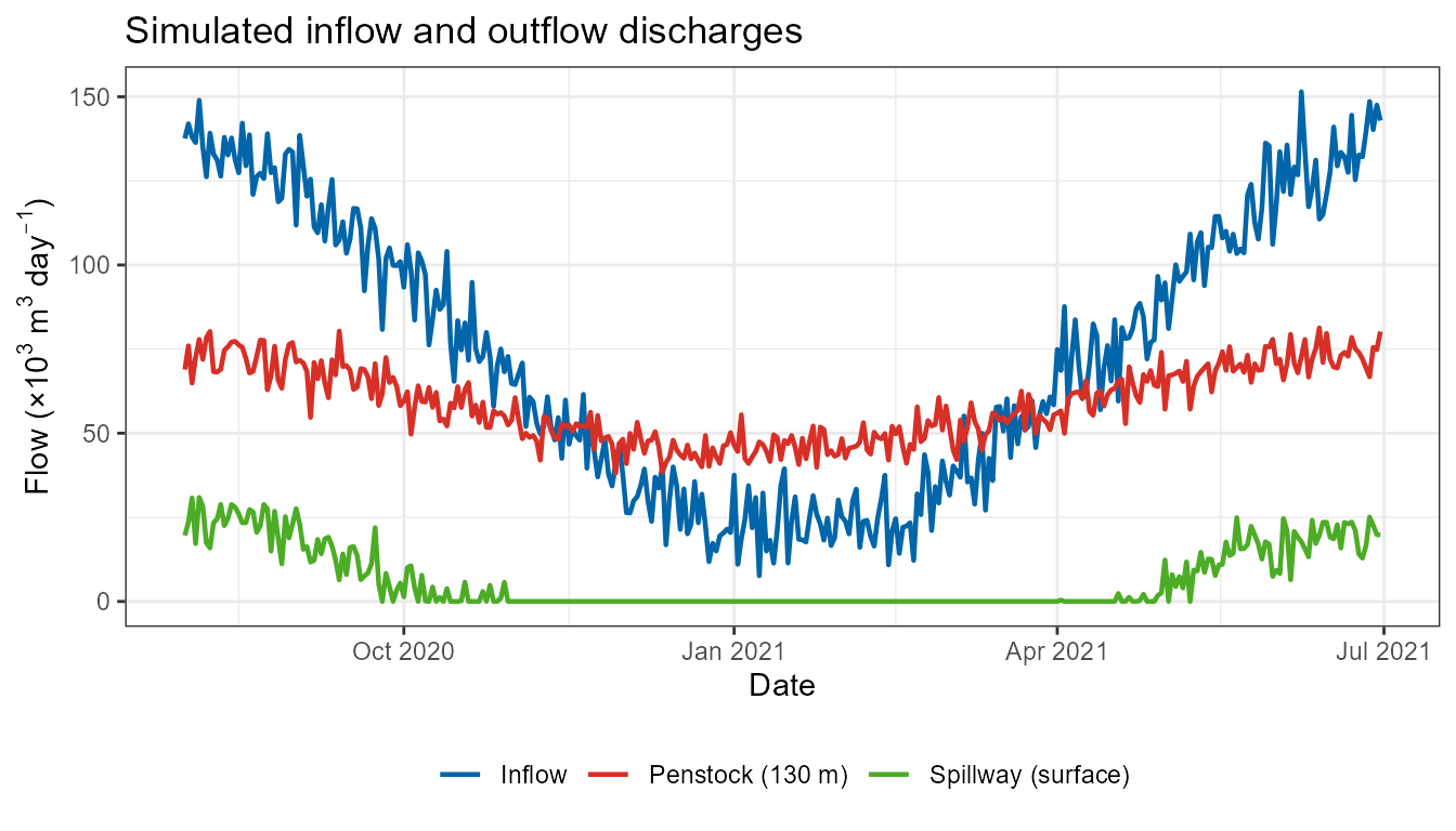

The penstock provides a near-constant regulated release throughout the year, while the spillway flows only during the high-flow winter months.

Outlet positions on the hypsograph

It is important that each subsurface outlet elevation falls within the elevation range of the hypsograph. Below we illustrate where the two outlets sit relative to the reservoir hypsograph.

outlet_lines <- data.frame(
  elev  = c(130, max(hypsograph$elev)),
  label = c("Penstock (130 m)", "Spillway (surface)")
)

ggplot(hypsograph, aes(x = area / 1e6, y = elev)) +
  geom_ribbon(aes(xmin = 0, xmax = area / 1e6), fill = "#cce5f7", alpha = 0.6) +
  geom_line(linewidth = 1, colour = "#0065a9") +
  geom_hline(data = outlet_lines,
             aes(yintercept = elev, colour = label),
             linetype = "dashed", linewidth = 0.9) +
  scale_colour_manual(
    values = c("Penstock (130 m)"   = "#d73027",
               "Spillway (surface)" = "#4dac26"),
    name = "Outlet"
  ) +
  labs(
    x     = expression("Area (km"^2 * ")"),
    y     = "Elevation (m a.s.l.)",
    title = "Outlet positions on reservoir hypsograph"
  ) +
  theme_bw() +
  theme(legend.position = "bottom")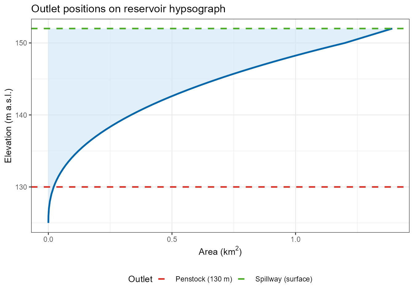

Build the AEME object

We assemble the AEME object with aeme_constructor(). The input list must include at minimum the hypsograph, meteorological data, and light extinction coefficient (Kw).

input <- list(
  init_depth = depth,
  hypsograph = hypsograph,
  meteo      = met,
  use_lw     = TRUE,
  Kw         = 0.5   # light extinction coefficient (m⁻¹)
)

aeme <- aeme_constructor(
  lake  = reservoir,
  time  = time,
  input = input
)
#> Time step missing. Setting time step to 3600 seconds.
#> Spin up for models missing. Setting spin up to 2 for all models.
aeme
#>             AEME 
#> -------------------------------------------------------------------
#>   Lake
#> Reservoir (ID: res001); Lat: -37.8; Lon: 176; Elev: 150m; Depth: 25m;
#> Area: 1200000 m2
#> -------------------------------------------------------------------
#>   Time
#> Start: 2020-08-01; Stop: 2021-06-30; Time step: 3600
#>  Spin up (days): GLM: 2; GOTM: 2; DYRESM: 2
#> -------------------------------------------------------------------
#>   Configuration
#>     Model controls: Absent 
#>     Use biogeochemical model: No
#>           Physical   |   Biogeochemical
#> DY-CD    : Absent     |   Absent 
#> GLM-AED  : Absent     |   Absent 
#> GOTM-WET : Absent     |   Absent 
#> -------------------------------------------------------------------
#>   Observations
#> Lake: Absent; Level: Absent
#> -------------------------------------------------------------------
#>   Input
#> Inital profile: Absent; Inital depth: 25m; Hypsograph: Present (n=62);
#> Meteo: Present; Use longwave: TRUE; Kw: 0.5
#> -------------------------------------------------------------------
#>   Inflows
#> Data: Absent; Scaling factors: DY-CD: 1; GLM-AED: 1; GOTM-WET: 1
#> -------------------------------------------------------------------
#>   Outflows
#> Data: Absent; Scaling factors: DY-CD: 1; GLM-AED: 1; GOTM-WET: 1
#> -------------------------------------------------------------------
#>   Water balance
#> Method: 2; Use: obs; Modelled: Absent; Water balance: Absent
#> -------------------------------------------------------------------
#>   Parameters: 
#> Number of parameters: 0
#> -------------------------------------------------------------------
#>   Output: 
#> 
#> DY-CD:    
#> GLM-AED:  
#> GOTM-WET:

Add inflows

Inflows are added as a named list of data frames. The name (here "river") is used as the stream identifier in each model.

aeme <- add_inflows(aeme, data = list(river = inflow_data))

Add multiple outflows

The add_outflows() function accepts:

data – a named list of outflow data frames (each with at least Date and HYD_flow columns).
elevation – a named list matching the names in data.
Use elevation = -1 for a surface outlet; supply the elevation in metres above sea level (within the hypsograph range) for a subsurface outlet.

aeme <- add_outflows(
  aeme,
  data = list(
    penstock = penstock_data,
    spillway = spillway_data
  ),
  elevation = list(
    penstock = 130,   # 20 m below the full supply level
    spillway = -1     # surface outlet (overflow)
  )
)

# Inspect the outflows slot
outf <- outflows(aeme)
cat("Outflow names :", paste(names(outf$data),      collapse = ", "), "\n")
#> Outflow names : penstock, spillway
cat("Elevations    :",
    paste(names(outf$elevation),
          unlist(outf$elevation), sep = " = ", collapse = "; "), "\n")
#> Elevations    : penstock = 130; spillway = -1

Printing the aeme object now shows both outlets registered in the outflows slot:

aeme
#>             AEME 
#> -------------------------------------------------------------------
#>   Lake
#> Reservoir (ID: res001); Lat: -37.8; Lon: 176; Elev: 150m; Depth: 25m;
#> Area: 1200000 m2
#> -------------------------------------------------------------------
#>   Time
#> Start: 2020-08-01; Stop: 2021-06-30; Time step: 3600
#>  Spin up (days): GLM: 2; GOTM: 2; DYRESM: 2
#> -------------------------------------------------------------------
#>   Configuration
#>     Model controls: Absent 
#>     Use biogeochemical model: No
#>           Physical   |   Biogeochemical
#> DY-CD    : Absent     |   Absent 
#> GLM-AED  : Absent     |   Absent 
#> GOTM-WET : Absent     |   Absent 
#> -------------------------------------------------------------------
#>   Observations
#> Lake: Absent; Level: Absent
#> -------------------------------------------------------------------
#>   Input
#> Inital profile: Absent; Inital depth: 25m; Hypsograph: Present (n=62);
#> Meteo: Present; Use longwave: TRUE; Kw: 0.5
#> -------------------------------------------------------------------
#>   Inflows
#> Data: Present; Scaling factors: DY-CD: 1; GLM-AED: 1; GOTM-WET: 1
#> -------------------------------------------------------------------
#>   Outflows
#> Data: Present; Scaling factors: DY-CD: 1; GLM-AED: 1; GOTM-WET: 1
#> -------------------------------------------------------------------
#>   Water balance
#> Method: 2; Use: obs; Modelled: Absent; Water balance: Absent
#> -------------------------------------------------------------------
#>   Parameters: 
#> Number of parameters: 0
#> -------------------------------------------------------------------
#>   Output: 
#> 
#> DY-CD:    
#> GLM-AED:  
#> GOTM-WET:

Build model configurations

build_aeme() translates the AEME object into the configuration files required by each model. Each model handles multiple outlets in its own way:

GLM-AED: creates individual CSV boundary condition files (bcs/outflow_<name>.csv) and sets num_outlet, outl_elvs, and outlet_type in glm3.nml.
GOTM-WET: creates individual data files (inputs/outf_<name>.dat) and updates gotm.yaml.
DYRESM-CAEDYM: writes all outlets into a single .wdr file with a column per outlet and the number of outlets in the header.

model_controls <- get_model_controls()
model          <- c("glm_aed")
path           <- file.path(tempdir(), "reservoir")

aeme <- build_aeme(
  aeme           = aeme,
  model          = model,
  model_controls = model_controls,
  path           = path,
  ext_elev       = 2,
  use_bgc        = FALSE,
  wb_method = 1
)
#> Created missing directory:
#> C:\Users\RUNNER~1\AppData\Local\Temp\Rtmpy8xaAe\reservoir
#> ℹ No water level present. Using constant water level.
#> ℹ Insufficient lake temperature observations to estimate surface temperature.
#>   Using Stefan & Preud'homme (2007) method.
#> ℹ No water balance correction applied (method = 1).
#> ℹ Calculating lake level using lake depth and a sinisoidal function.
#> ℹ Building GLM-AED for lake reservoir
#> ℹ Copied in GLM nml file
#> ℹ Copied in AED nml file and supporting files
#> ✔ GLM nml validation completed - no issues detected.

Run the models

aeme <- run_aeme(aeme = aeme, model = model, path = path)
#> ℹ Running models... (Have you tried parallelizing?) [2026-03-31 01:05:40]
#> → GLM-AED running... [2026-03-31 01:05:40]
#> ✔ GLM-AED run successful! [2026-03-31 01:05:41]
#> ✔ Model run complete! [2026-03-31 01:05:41]

View the output

plot_output(aeme = aeme)
#> Warning: Removed 124 rows containing missing values or values outside the scale range
#> (`geom_col()`).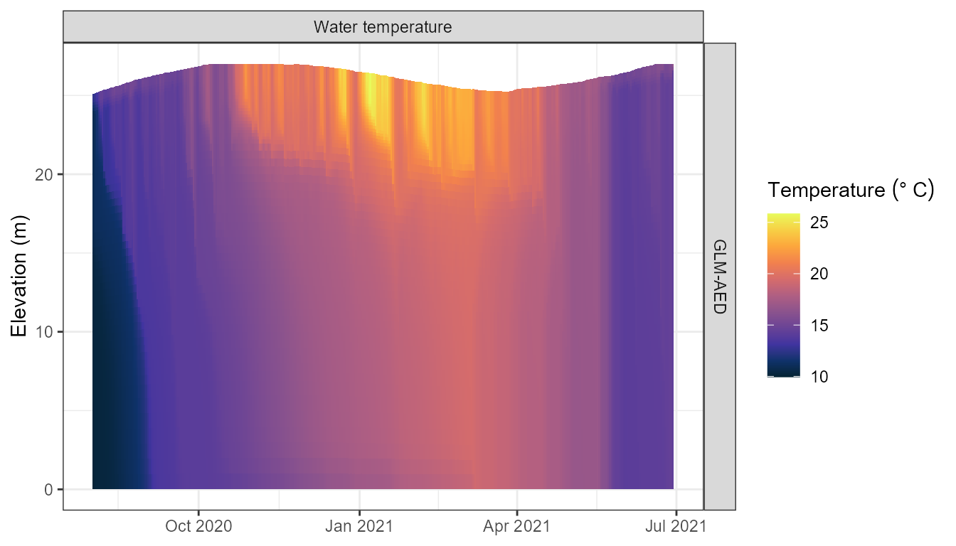

Summary

This vignette has shown how to configure AEME for a reservoir with multiple outlets at different elevations. The key steps are:

Define the reservoir geometry using a more prismatic hypsograph (volume_development > 1.5) appropriate for a constructed reservoir.
Create time series for each inflow and each outlet independently.
Register multiple outlets with add_outflows(), providing a named data list and a matching named elevation list. Use elevation = -1 for a surface outlet; provide the actual elevation (m a.s.l.) for subsurface outlets, ensuring values fall within the hypsograph elevation range.
Build and run the model ensemble with build_aeme() and run_aeme().

Currently only one of the three hydrodynamic models, GLM-AED, supported by AEME (DYRESM-CAEDYM, GLM-AED, and GOTM-WET) can handle multiple outlets and produce separate outlet files during the build step, allowing each outlet’s contribution to be tracked independently.