Rotoehu - Merge Bathymetry with DEM data • bathytools

Lake bathymetry data is useful for a range of applications, including habitat mapping, water quality monitoring, and hydrodynamic modelling. However, lakes sit within a landscape, and it is often useful to know how the bathymetry data relates to the surrounding topography. This is particularly important for hydrodynamic modelling of lakes with large fluctuations in water level, or for flood risk assessments in the surrounding area.

This vignette demonstrates how to merge bathymetry data with a Digital Elevation Model (DEM) raster using the merge_bathy_dem() function.

Load the data

We will use the bathytools package to merge bathymetry data with a DEM raster. The package includes example data for Lake Rotoehu, New Zealand. The bathymetry data is stored as a a contour shapefile accessible via the Limnotrack ltapi package. Whereas the DEM data is stored as a raster in a TIF file. The DEM raster was prepared from LiDAR data provided by Land Information New Zealand and aggregated to 32m. The original 1m data can be downloaded here.

We will also use a shapefile of the lake shoreline and a shapefile of the lake catchment. These are both sourced from the LERNZmp database. The LERNZmp database was developed as part of the LERNZmp project. Read more about the LERNZmp project here or visit the Shiny platform here.

library(bathytools)
library(tmap) # Used for plotting spatial data

# Lake Rotoehu lake id is 40188
shoreline <- ltapi::lt_fetch(
  "lernzmp_lakes",
  filter = ltapi::lt_filter(lernzmp_id == "LID40188")
)
# Get lake catchment
catchment <- ltapi::lt_fetch(
  "lernzmp_catchments",
  filter = ltapi::lt_filter(lernzmp_id == "LID40188")
)

# The catchment shapefile is in WGS84 (EPSG:4326) but the data is in NZTM2000 
# (EPSG:2193). We will set the CRS of the catchment to NZTM2000.
sf::st_crs(catchment) <- 2193
#> Warning: st_crs<- : replacing crs does not reproject data; use st_transform for
#> that

The example lake we will be looking at is Lake Rotoehu in the Bay of Plenty Region on the North Island of Aotearoa New Zealand.

The tmap package is used to plot spatial data. The tmap_mode("view") function is used to display the map in the viewer pane in RStudio. The tmap_options(basemaps = "Esri.WorldImagery") function is used to set the basemap to a satellite image. It is similar to the ggplot2 package, but is specifically designed for spatial data. Here we plot the lake shoreline in light blue and the lake catchment in pink.

tmap_mode("view")
#> ℹ tmap modes "plot" - "view"
#> ℹ toggle with `tmap::ttm()`
tmap_options(basemap.server = "Esri.WorldImagery")

tm_shape(shoreline) +
  tm_borders(col = "#8DA0CB", lwd = 2) +
  tm_shape(catchment) +
  tm_borders(col = "#E78AC3", lwd = 2)

The depth data is stored as contours and is available on the same LERNZmp database. The depth contours are stored as a shapefile and can be accessed using the ltapi package. The depth contours are in meters and are negative values. We will convert the depth contours to positive values for plotting.

# Get lake depth contours
contours  <- ltapi::lt_fetch(
  "lake_contours",
  filter = ltapi::lt_filter(lernzmp_id == "LID40188")
) |>
  dplyr::mutate(depth = depth_m)

dem_raster <- terra::rast(system.file("extdata/dem_32m.tif",
                                      package = "bathytools"))
tm_shape(dem_raster) +
  tm_raster(col_alpha = 0.5, col.scale = tm_scale_continuous(values = "-brewer.yl_gn_bu")) +
  tm_shape(shoreline) +
  tm_borders(col = "#FC8D62", lwd = 2) +
  tm_shape(catchment) +
  tm_borders(col = "#A6D854", lwd = 2)

Generate the bathymetry raster

The first step is to generate a bathymetry raster from the shoreline and depth data. The rasterise_bathy() function is used to generate the bathymetry raster. The function takes the shoreline, depth data, and the coordinate reference system (CRS) as inputs. The function returns a SpatRaster object representing the bathymetry raster.


bathy_raster <- rasterise_bathy(shoreline = shoreline,
                                contours = contours,
                                crs = 2193,
                                res = 8)
#> No islands found.
#> ℹ Generating depth points for interpolation
#> Warning in st_cast.sf(p[!sf::st_is_empty(p$geometry), ], "POINT"): repeating
#> attributes for all sub-geometries for which they may not be constant
#> Warning in st_cast.sf(p[!sf::st_is_empty(p$geometry), ], "POINT"): repeating
#> attributes for all sub-geometries for which they may not be constant
#> Warning in st_cast.sf(p[!sf::st_is_empty(p$geometry), ], "POINT"): repeating
#> attributes for all sub-geometries for which they may not be constant
#> Warning in st_cast.sf(p[!sf::st_is_empty(p$geometry), ], "POINT"): repeating
#> attributes for all sub-geometries for which they may not be constant
#> Warning in st_cast.sf(p[!sf::st_is_empty(p$geometry), ], "POINT"): repeating
#> attributes for all sub-geometries for which they may not be constant
#> Warning in st_cast.sf(p[!sf::st_is_empty(p$geometry), ], "POINT"): repeating
#> attributes for all sub-geometries for which they may not be constant
#> Warning: large number of points for interpolation (95645)
#> ✔ Generating depth points for interpolation [6.2s]
#> 
#> ℹ Interpolating depth points to raster
#> ℹ Adjusting depths >= 0 to -0.4m
#> ℹ Interpolating depth points to raster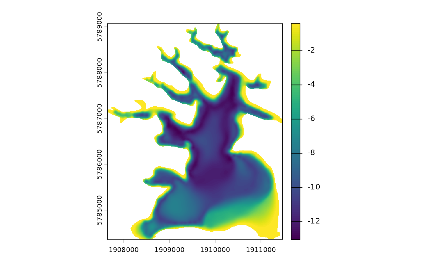

#> ✔ Interpolating depth points to raster [870ms]

tm_shape(dem_raster) +
  tm_raster(col_alpha = 0.5, 
            col.scale = tm_scale_continuous(values = "-brewer.yl_gn_bu")) +
  tm_shape(bathy_raster) +
  tm_raster(col.scale = tm_scale_continuous(values = "-viridis", ticks = seq(-90, 0, by = 10))) +
  tm_shape(shoreline) +
  tm_borders(col = "#FC8D62", lwd = 2) +
  tm_shape(catchment) +
  tm_borders(col = "#A6D854", lwd = 2)

Merge the bathymetry with the DEM

The next step is to merge the bathymetry raster with the DEM raster. The merge_bathy_dem() function is used to merge the bathymetry raster with the DEM raster. The function takes the shoreline, bathymetry raster, DEM raster, and catchment shapefile as inputs. The function returns a SpatRaster object representing the merged bathymetry and DEM data.

If the resolution of the bathymetry raster is different from the DEM raster, the bathymetry raster will be resampled to match the resolution of the DEM raster.


dem_bath <- merge_bathy_dem(shoreline = shoreline, bathy_raster = bathy_raster,
                            dem_raster = dem_raster, catchment = catchment)
#> Resolutions differ. Resampling bathy_raster to DEM resolution.
#> Lake surface elevation from DEM: 294.25 m
dem_bath
#> class       : SpatRaster
#> size        : 338, 208, 1  (nrow, ncol, nlyr)
#> resolution  : 32, 32  (x, y)
#> extent      : 1906176, 1912832, 5778576, 5789392  (xmin, xmax, ymin, ymax)
#> coord. ref. : NZGD2000 / New Zealand Transverse Mercator 2000 (EPSG:2193)
#> source(s)   : memory
#> varname     : dem_32m
#> name        :  elevation
#> min value   : 281.262914
#> max value   : 644.796875

Spatial plot of the merged raster

Here we plot the merged raster with the lake and catchment boundaries.

tm_shape(dem_bath) +
  tm_raster(col_alpha = 0.5, 
            col.scale = tm_scale_continuous(values = "-brewer.yl_gn_bu")) +
  tm_shape(shoreline) +
  tm_borders(col = "#FC8D62", lwd = 2) +
  tm_shape(catchment) +
  tm_borders(col = "#A6D854", lwd = 2)

The colours in this plot do not clearly distinguish between the bathymetry and DEM data. We will add a break at the surface elevation of the lake to better distinguish between the two datasets. We can extract the water surface elevation from the DEM data using the get_lake_surface_elevation() function.

lake_elev <- get_lake_surface_elevation(dem_raster = dem_raster,
                                        shoreline = shoreline)
#> Lake surface elevation from DEM: 294.25 m

We can now plot the merged raster with the lake surface elevation as the break in the colour palette.

tm_dem_bath(dem_bath = dem_bath, lake_elev = lake_elev)

Hypsograph of the merged raster

A hypsograph is a plot of the area of a lake at different depths. The bathy_to_hypso() function can be used to generate a hypsograph from the bathymetry raster. The function takes the bathymetry raster as input and returns a data frame with the depth and area at each depth.


hyps <- bathy_to_hypso(bathy_raster = bathy_raster)
head(hyps)
#>   elev depth    area
#> 1  0.0   0.0 8089024
#> 2 -0.2  -0.2 7810453
#> 3 -0.4  -0.4 7531883
#> 4 -0.6  -0.6 7253312
#> 5 -0.8  -0.8 7157888
#> 6 -1.0  -1.0 7065600

The hypsograph can be plotted to show the area of the lake at different depths.

library(ggplot2)

ggplot(hyps, aes(x = area, y = depth)) +
  geom_line() +
  geom_point() +
  labs(x = "Area (m^2)", y = "Depth (m)") +
  theme_bw()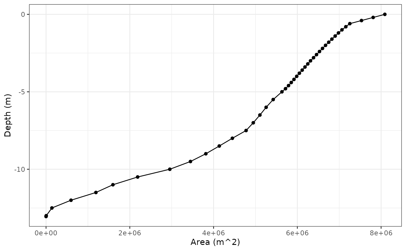

Extended hypsograph of the merged raster

When merging bathymetry with DEM data, it is often useful to extend the hypsograph to include the area of the lake at different elevations above the lake surface. This can be done by specifying an additional elevation to extend the lake surface. The dem_to_hypso() function can take an additional argument ext_elev to specify this elevation. It also requires the merged raster and the lake surface elevation as inputs, the lake shoreline polygon, and the lake elevation.

Here we will extend the hypsograph by 3 meters above the lake surface elevation. This will allow us to see the area of the lake at different elevations above the lake surface.


lake_depth <- get_lake_depth(bathy_raster = bathy_raster)
ext_hyps <- dem_to_hypsograph(shoreline = shoreline, dem_bath = dem_bath, 
                              lake_elev = lake_elev, lake_depth = lake_depth,
                              ext_elev = 3)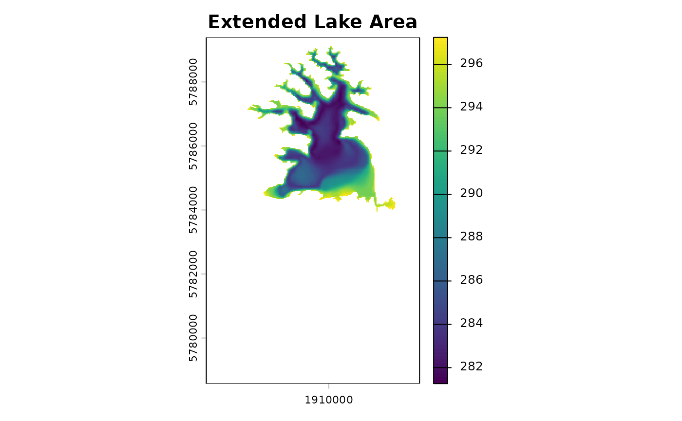

head(ext_hyps)
#>     elev depth    area
#> 1 297.25   3.0 9153536
#> 2 297.05   2.8 9097216
#> 3 296.85   2.6 9032704
#> 4 296.65   2.4 8966144
#> 5 296.45   2.2 8894464
#> 6 296.25   2.0 8838144

The extended hypsograph can be plotted to show the area of the lake at different depths or elevations. Here we will plot the area of the lake at different elevations above the lake surface.


ggplot(ext_hyps, aes(x = area, y = elev)) +
  geom_hline(yintercept = lake_elev, linetype = "dashed", color = "red") +
  geom_line() +
  geom_point() +
  labs(x = "Area (m^2)", y = "Elevation (m.a.s.l)") +
  theme_bw()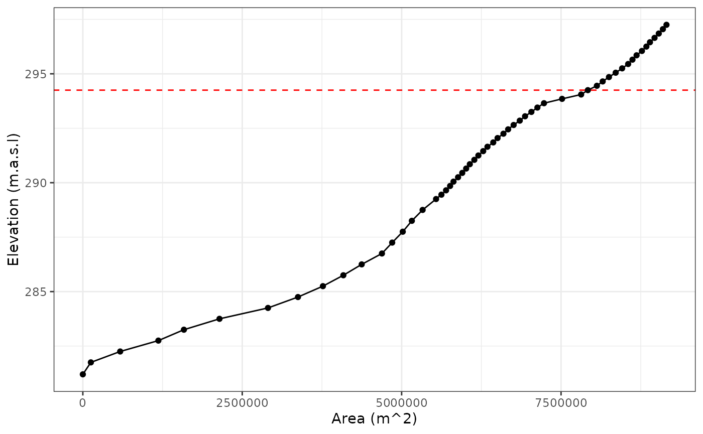

3-D plot of the merged raster

The plot_raster_3d() function can be used to create a 3-D plot of the merged raster. The function takes the merged raster and the shoreline as inputs. The fact argument controls the aggregation factor for the raster. A higher factor will result in a smoother plot, but will take longer to render.

p1 <- plot_raster_3d(x = dem_bath, shoreline = shoreline, split_lake = TRUE)
p1

Saving the merged raster

The merged raster can be saved to a file using the terra::writeRaster() function. The function takes the raster object and the file path as inputs.

It is important to note that SpatRaster can not be saved as “.rds” files. They can also be quite large, so it is recommended to save the raster in a compressed format, such as GeoTIFF.

terra::writeRaster(dem_bath, "dem_bath.tif", overwrite = TRUE)