library(aemetools)
library(sf)
library(terra)
library(tmap)
tmap_mode("view")
tmap_options(basemap.server = "OpenTopoMap")
Global
Download global point meteorological data
One of the most widely used meteorological datasets for hydrodynamic modelling is the ERA5-Land reanalysis dataset. This dataset has a spatial resolution of ~9 km and provides hourly meteorological data for the period 1950-present. It also includes a wide range of meteorological variables that are required to drive hydrological and hydrodynamic models.
However, there are known issues with the ERA5-Land dataset, such as the underestimation of precipitation and wind speed in some regions. Therefore, it is recommended to compare the ERA5-Land data with local observations before using it for hydrodynamic modelling.
Set up Copernicus (CDS) account and link with ecmwfr
package
Please see instructions on setting up a Copernicus (CDS) account and
linking it with the ecmwfr package in the ecmwfr
vignette.
key <- "XXXXXXXX-XXXX-XXXX-XXXX-XXXXXXXXXXXX"
user <- "person@email.com"

# Add the key and user to the environment
Sys.setenv(CDS_KEY = key)
Sys.setenv(CDS_USER = user)

# Set the key for connecting to Copernicus Data Store (CDS)
ecmwfr::wf_set_key(key = Sys.getenv("CDS_KEY"),
                   user = Sys.getenv("CDS_USER"))
Download ERA5 data
Point timeseries data
The get_era5_isimip_point() function can be used to
download ERA5 meteorological data for a specific point location. This
uses the ISIMIP3a dataset which is a subset of the ERA5 dataset and is
accessed via the ISIMIP
API. This function requires the latitude, longitude, years, and
variables to be specified. It can be used for any point location
globally. However, this dataset only covers 1900-2021.
Example: Download meterological data for 2021 for Lake Toba, Indonesia
However, it is very quick and easy to download meteorological data for a specific point location. We will choose the latitude and longitude of Lake Toba, Indonesia, and download the air temperature and precipitation for the year 2021.
lon <- 98.67591
lat <- 2.637047
years <- 2021
vars <- c("MET_tmpair", "MET_pprain")

met <- get_era5_isimip_point(lon, lat, years, vars)
#> INFO [2026-06-17 00:05:15] job submitted
#> INFO [2026-06-17 00:05:15] downloading
#> INFO [2026-06-17 00:05:16] extracting
summary(met)
#>       Date              MET_tmpair      MET_pprain
#>  Min.   :2021-01-01   Min.   :19.08   Min.   : 0.06125
#>  1st Qu.:2021-04-02   1st Qu.:21.29   1st Qu.: 1.88049
#>  Median :2021-07-02   Median :21.79   Median : 4.86638
#>  Mean   :2021-07-02   Mean   :21.77   Mean   : 7.66636
#>  3rd Qu.:2021-10-01   3rd Qu.:22.30   3rd Qu.:10.38196
#>  Max.   :2021-12-31   Max.   :23.67   Max.   :68.75736
GRIB files
The download_era5_grib() function can be used to
download ERA5 meteorological data from the Copernicus Data Store (CDS).
This function requires the latitude, longitude, variable, year, and
month to be specified. The data will be saved as a GRIB file in the
specified path.
Download shapefile for Lake Toba, Indonesia
We will download a shapefile for Lake Toba, Indonesia, and plot the
location using the osmdata and tmap
packages.
For more details on using osmdata, you can visit the osmdata website.
library(osmdata)
osm_data <- opq(bbox = "Sumatra, Indonesia") |>
  add_osm_feature(key = "name:en", value = "Lake Toba", value_exact = FALSE) |>
  osmdata_sf()

# Extract lake polygon
toba <- osm_data$osm_multipolygons |>
  st_make_valid()
toba
Sometimes the osmdata package can be a bit tricky to use
and may get rate limit errors from the OpenStreetMap API. An alternative
is to use the Nominatim API to download the shapefile for Lake Toba.
This can be done using the st_read() function.
Plot the location of Lake Toba.
tm_shape(toba) +
  tm_fill(fill = "blue", fill_alpha = 0.5) +
  tm_borders(col = "black")
Alternatively, you can manually input the latitude and longitude of the location you are interested in.
lat <- 2.637047
lon <- 98.67591

# View location
coords <- data.frame(lat = lat, lon = lon) |>
  st_as_sf(coords = c("lon", "lat"), crs = 4326)

tm_shape(coords) +
  tm_dots(fill = "red", size = 2)
Now we can download the ERA5 data for the 2m temperature for January
2024. We can use the download_era5_grib() function to
download the data using the shapefile we downloaded earlier or the
latitude and longitude of the location.
year <- 2024
month <- 1
variable <- "2m_temperature"
path <- "data/test"
site <- "toba"

files <- download_era5_grib(shape = toba, year = year, month = month,
                            variable = variable, path = path, site = site,
                            user = user)
The function will return the path to the downloaded file.
files
#> [1] "data/test/reanalysis-era5-land_2m_temperature_hourly_2024_1_toba.grib"
Files are in GRIB (GRIdded Binary) format, which is a format commonly used in meteorology to store gridded data. You can read more about these files on the ECMWF website: GRIB.
The most important thing is not to be afraid of them. You can easily
read them using the terra::rast() function.
r <- rast(files[1])
r
#> class       : SpatRaster
#> size        : 8, 8, 744  (nrow, ncol, nlyr)
#> resolution  : 0.1, 0.1  (x, y)
#> extent      : 98.45, 99.25, 2.25, 3.05  (xmin, xmax, ymin, ymax)
#> coord. ref. : lon/lat Coordinate System imported from GRIB file
#> source      : reanalysis-era5-land_2m_temperature_hourly_2024_1_toba.grib
#> names       : SFC (~e [C], SFC (~e [C], SFC (~e [C], SFC (~e [C], SFC (~e [C], SFC (~e [C], ...
#> unit        : C
#> time        : 2024-01-01 00:00:00 to 2024-01-31 23:00:00 (744 steps)
Hmmmmmmm… Ok, maybe these files are not that easy to read/understand.
We can also plot them in leaflet using the terra::plet()
function.
plet(r)As you can see it gives us a spatial grid of the 2m temperature for
the month of January 2024. However it is at a 1-hour temporal
resolution. We can use the read_grib_point() function to
extract the timeseries data at a specific point location.
df <- read_grib_point(file = files, shape = toba)
head(df)
#>              DateTime    value units
#> 1 2024-01-01 00:00:00 293.0246     C
#> 2 2024-01-01 01:00:00 293.3110     C
#> 3 2024-01-01 02:00:00 293.9233     C
#> 4 2024-01-01 03:00:00 294.9492     C
#> 5 2024-01-01 04:00:00 296.1867     C
#> 6 2024-01-01 05:00:00 297.0911     C
#>                                                 variable short_name
#> 1 SFC (Ground or water surface); 2 metre temperature [C]         2T
#> 2 SFC (Ground or water surface); 2 metre temperature [C]         2T
#> 3 SFC (Ground or water surface); 2 metre temperature [C]         2T
#> 4 SFC (Ground or water surface); 2 metre temperature [C]         2T
#> 5 SFC (Ground or water surface); 2 metre temperature [C]         2T
#> 6 SFC (Ground or water surface); 2 metre temperature [C]         2T
New Zealand
Download NZ point meteorological data
Currently, there are ERA5-Land data (~9km grid spacing) archived for New Zealand (166.5/-46.6/178.6/-34.5) for the time period 1980-2023 with the main meteorological variables (air temperature, dewpoint temperature, wind u-vector at 10m, wind v-vector at 10m, total precipitation, snowfall, surface level pressure, downwelling shortwave radiation, downwelling longwave radiation) required to drive hydrological and hydrodynamic models. This can be easily downloaded using the example below.
First we will define our point location for New Zealand. We will use the latitude and longitude of Lake Rotorua, Bay of Plenty, New Zealand.
lon <- 176.2717
lat <- -38.079
Plot the location.
coords <- data.frame(lat = lat, lon = lon) |>
  st_as_sf(coords = c("lon", "lat"), crs = 4326)

tm_shape(coords) +
  tm_dots(fill = "red", size = 2)
Now we can download the ERA5 data for the air temperature and
precipitation for the years 2000-2001. We can use the
get_era5_land_point_nz() function to download the data.
The function will return a dataframe with the daily meteorological data for the specified years.
vars <- c("MET_tmpair", "MET_pprain")

met <- get_era5_land_point_nz(lat = lat, lon = lon, years = 2000:2001,
                              vars = vars)
summary(met)
#>       Date              MET_tmpair       MET_pprain
#>  Min.   :2000-01-01   Min.   : 3.567   Min.   : 0.0000
#>  1st Qu.:2000-07-01   1st Qu.: 9.178   1st Qu.: 0.1464
#>  Median :2000-12-31   Median :12.053   Median : 1.5939
#>  Mean   :2000-12-31   Mean   :11.967   Mean   : 6.3207
#>  3rd Qu.:2001-07-01   3rd Qu.:14.835   3rd Qu.: 6.9353
#>  Max.   :2001-12-31   Max.   :19.837   Max.   :89.4112
We can plot the timeseries data using the ggplot2
package.
library(ggplot2)
library(tidyr)
#>
#> Attaching package: 'tidyr'
#> The following object is masked from 'package:terra':
#>
#>     extract

met |>
  pivot_longer(cols = c(MET_tmpair, MET_pprain)) |>
  ggplot(aes(x = Date, y = value)) +
  geom_line() +
  facet_wrap(~name, scales = "free_y", ncol = 1) +
  theme_bw()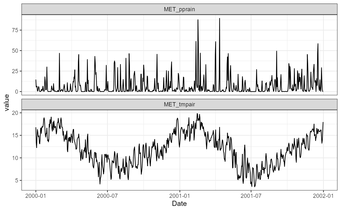
By default, it will download all available variables. Currently
available variables are air temperature (MET_tmpair), dew
point temperature (MET_tmpdew), wind u-component
(MET_wnduvu), wind v-component (MET_wnduvv),
precipitation (MET_pprain), snowfall
(MET_ppsnow), surface level pressure
(MET_prsttn) and shortwave radiation
(MET_radswd).
To download all available variables for Lake Rotorua for the years 2022-2023, you can use the following code:
met <- get_era5_land_point_nz(lat = lat, lon = lon, years = 2022:2023)
summary(met)
#>       Date              MET_tmpair       MET_tmpdew       MET_wnduvu
#>  Min.   :2022-01-01   Min.   : 4.725   Min.   :-2.106   Min.   :-5.5620
#>  1st Qu.:2022-07-02   1st Qu.: 9.901   1st Qu.: 6.845   1st Qu.:-1.3116
#>  Median :2022-12-31   Median :12.940   Median : 9.723   Median : 0.1794
#>  Mean   :2022-12-31   Mean   :12.899   Mean   : 9.755   Mean   : 0.2274
#>  3rd Qu.:2023-07-01   3rd Qu.:15.961   3rd Qu.:12.792   3rd Qu.: 1.8215
#>  Max.   :2023-12-31   Max.   :21.905   Max.   :21.368   Max.   : 5.7673
#>    MET_wnduvv         MET_pprain         MET_ppsnow          MET_prsttn
#>  Min.   :-4.82260   Min.   :  0.0000   Min.   :0.000e+00   Min.   :93756
#>  1st Qu.:-1.09642   1st Qu.:  0.1583   1st Qu.:0.000e+00   1st Qu.:96870
#>  Median : 0.18915   Median :  1.6596   Median :0.000e+00   Median :97352
#>  Mean   : 0.07119   Mean   :  8.1192   Mean   :1.521e-16   Mean   :97314
#>  3rd Qu.: 1.25388   3rd Qu.: 10.5166   3rd Qu.:0.000e+00   3rd Qu.:97879
#>  Max.   : 5.16590   Max.   :106.9180   Max.   :3.470e-15   Max.   :99473
#>    MET_radswd
#>  Min.   :  8.615
#>  1st Qu.: 93.090
#>  Median :150.059
#>  Mean   :164.618
#>  3rd Qu.:229.137
#>  Max.   :386.774
Derive other meteorological variables
The downloaded ERA5 data can be converted to other meteorological
variables using the AEME::expand_met() function. Which will
calculate the following variables:
-
MET_tmpdew: Dew point temperature (°C) -
MET_wndspd: Wind speed (m/s) -
MET_wnddir: Wind direction (°) -
MET_radlwd: Longwave radiation (W/m²) -
MET_cldcvr: Cloud cover (fraction) -
MET_prmslp: Mean sea level pressure (Pa) -
MET_humrel: Relative humidity (%) -
MET_prvapr: Vapour pressure (Pa)
To use this function, you will need to provide the latitude, longitude, and elevation of the site. Elevation is required to calculate the mean sea level pressure and cloud cover.
We can access the elevation data using the
get_dem_value() function. This function uses the LINZ data
service to obtain the elevation value for a given latitude and longitude
using the national 8m digital elevation model (DEM) layer (ID:
51768).
This requires a LINZ API key which can be obtained by visiting the LINZ
website and registering for an account. Then adding it to your R
session using the add_linz_key() function.
elev <- get_dem_value(lat = lat, lon = lon)
elev
#> [1] 282
Now we can expand the meteorological data to include the derived variables.
met <- AEME::expand_met(met, lat = lat, lon = lon, elev = elev)
#> Warning in sqrt((1 - df$swr/df$Ho)/0.65): NaNs produced
summary(met)
#>       Date              MET_radswd        MET_radlwd      MET_cldcvr
#>  Min.   :2022-01-01   Min.   :  8.615   Min.   :186.7   Min.   :0.1580
#>  1st Qu.:2022-07-02   1st Qu.: 93.090   1st Qu.:248.6   1st Qu.:0.5600
#>  Median :2022-12-31   Median :150.059   Median :288.2   Median :0.7300
#>  Mean   :2022-12-31   Mean   :164.618   Mean   :291.7   Mean   :0.7058
#>  3rd Qu.:2023-07-01   3rd Qu.:229.137   3rd Qu.:332.2   3rd Qu.:0.8738
#>  Max.   :2023-12-31   Max.   :386.774   Max.   :410.8   Max.   :1.0000
#>    MET_tmpair       MET_humrel      MET_tmpdew       MET_prvapr
#>  Min.   : 4.725   Min.   :50.18   Min.   :-2.106   Min.   : 5.242
#>  1st Qu.: 9.901   1st Qu.:74.78   1st Qu.: 6.845   1st Qu.: 9.918
#>  Median :12.941   Median :82.01   Median : 9.723   Median :12.059
#>  Mean   :12.899   Mean   :81.77   Mean   : 9.755   Mean   :12.455
#>  3rd Qu.:15.961   3rd Qu.:89.29   3rd Qu.:12.792   3rd Qu.:14.781
#>  Max.   :21.905   Max.   :99.71   Max.   :21.368   Max.   :25.445
#>    MET_prsttn      MET_prmslp       MET_wndspd      MET_wnddir
#>  Min.   :93756   Min.   : 96901   Min.   :0.079   Min.   :  0.909
#>  1st Qu.:96870   1st Qu.:100164   1st Qu.:1.517   1st Qu.: 77.121
#>  Median :97352   Median :100663   Median :2.375   Median :168.021
#>  Mean   :97314   Mean   :100637   Mean   :2.502   Mean   :173.417
#>  3rd Qu.:97879   3rd Qu.:101219   3rd Qu.:3.388   3rd Qu.:261.986
#>  Max.   :99473   Max.   :102904   Max.   :7.405   Max.   :358.476
#>    MET_wnduvu        MET_wnduvv        MET_pprain         MET_ppsnow
#>  Min.   :-5.5620   Min.   :-4.8230   Min.   :  0.0000   Min.   :0
#>  1st Qu.:-1.3120   1st Qu.:-1.0967   1st Qu.:  0.1585   1st Qu.:0
#>  Median : 0.1795   Median : 0.1890   Median :  1.6595   Median :0
#>  Mean   : 0.2274   Mean   : 0.0712   Mean   :  8.1192   Mean   :0
#>  3rd Qu.: 1.8213   3rd Qu.: 1.2537   3rd Qu.: 10.5162   3rd Qu.:0
#>  Max.   : 5.7670   Max.   : 5.1660   Max.   :106.9180   Max.   :0
With these simple steps, you can download and derive meteorological data for your location of interest. This data can be used to drive hydrological and hydrodynamic models for your study area.
Head over to the AEME Inputs vignette to learn more about how to use the meteorological data to drive hydrodynamic models.