Once you have hourly ERA5-Land netCDF or GRIB on disk (see
vignette("download-era5")),
extract_era5_hourly_met() pulls a
metscale-shaped hourly series out of it for a point or a
polygon. extract_era5_lake_met() is a thin wrapper that
takes a lake polygon and defaults to the area-weighted method. The
extraction chunks here are not executed (they need the
reanalysis archive); the exceptions are reading the bundled lake polygon
and the grid visualisations near the end, which run against a small
synthesised grid.
library(metscale)
ex <- system.file("extdata", package = "metscale")
Point extraction
met <- extract_era5_hourly_met(
  path      = "era5_netcdf",          # directory of monthly hourly .nc files
  lon       = 176.2717,
  lat       = -38.0790,
  years     = 2023:2025,
  method    = "bilinear",             # 4 nodes around the point
  tz        = "Etc/GMT-12",
  format    = "AEME")                 # MET_* names and units
Files are located by matching pattern against the names
in path. The default, "{variable}", finds any
.nc / .grib file whose name holds the ERA5
variable name and a 4-digit year – enough for
download_era5_cds() output and most ad-hoc layouts. Give it
explicitly to disambiguate or to filter by month, e.g.
pattern = "{year}_{month}_{variable}" or
pattern = "*_{variable}_hourly_{year}_{month}_*";
{year} / {month} are optional and
* is a wildcard. variables defaults to the
nine ERA5-Land fields metscale needs;
precip_units and pressure_units control the
output units ("mm/hr" and "Pa" by default).
fill_gaps = TRUE reindexes onto a complete regular hourly
sequence.
Polygon (lake-average) extraction
A lake wider than an ERA5-Land grid cell (~0.1°, roughly 9 km at this
latitude) covers several cells, and a point sample then depends on
exactly where the point falls. Averaging over the cells that overlap the
lake polygon is more stable. Pass the geometry as geom:
lake_poly <- readRDS(file.path(ex, "rotorua_lake_shape.rds"))   # an sf polygon

met_area <- extract_era5_hourly_met(
  path   = "era5_netcdf",
  geom   = lake_poly,
  years  = 2023:2025,
  method = "area",                    # area-weighted mean of overlapping cells
  tz     = "Etc/GMT-12")
method chooses the spatial sampling:
method |
what it does | use when |
|---|---|---|
"nearest" |
single closest cell centre | lake well inside one cell |
"bilinear" |
4 cell centres around the centroid | point-like water body (default) |
"area_mean" |
unweighted mean of cells overlapping the polygon | lake spans a few cells |
"area" |
area-weighted mean of overlapping cells | lake spans several cells unevenly |
The bundled Lake Rotorua polygon spans more than one cell, so
"area" is the right choice:
lake_poly <- readRDS(file.path(ex, "rotorua_lake_shape.rds"))
sf::st_crs(lake_poly)$epsg          # 2193 (NZTM); any CRS is accepted
#> [1] 2193
round(as.numeric(sum(sf::st_area(lake_poly))) / 1e6, 1)   # lake area, km^2
#> [1] 82
sf::st_bbox(sf::st_transform(lake_poly, 4326))            # ~0.11 deg E-W
#>      xmin      ymin      xmax      ymax
#> 176.21613 -38.14151 176.32674 -38.03251
An ~0.11° east–west extent against a ~0.1° grid means the lake touches two to three cells in each direction — exactly the case area-weighting is for.
Visualising the grid and the sampling
plot_extract_grid() reads the same files an extraction
would and draws the point or polygon against the ERA5-Land grid, shading
the cells the chosen method samples by their weight. Run it
before an extraction to confirm the geometry sits where you expect — a
shapefile in the wrong projection or a sign-flipped longitude jumps out
on the map and nowhere else.
The package ships only the extracted series, so the chunks below
synthesise a bare ERA5-Land grid (regular 0.1°) over the lake; against
real files on disk the plot_extract_grid() calls are
identical.
A point, "bilinear"
For lon / lat (or a small water body)
plot_extract_grid() shows the four nodes the bilinear blend
uses and their weights.
plot_extract_grid(gdir, lon = 176.2717, lat = -38.0790, method = "bilinear")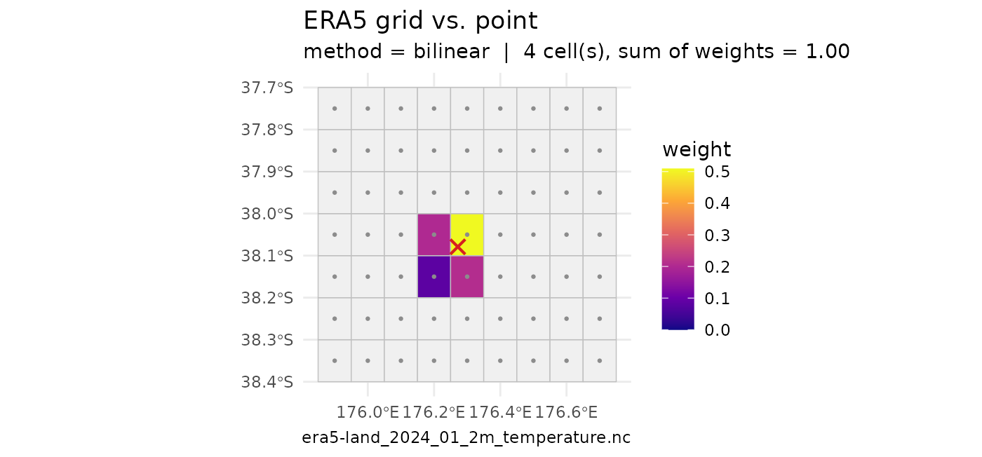
Figure 1. A point (red cross) with
method = "bilinear": the four surrounding grid cells,
weighted by proximity (weights sum to 1). "nearest" would
keep only the single closest of them. The subtitle reports the method,
the cell count and (for a one-cell sample) the point-to-centre distance.
The four method options on the lake polygon
The same Lake Rotorua outline under each method from the
table above. The returned object is a ggplot carrying the
drawn cells as an sf on attr(., "grid")
(columns ix, iy, weight,
selected, land), so the four can be pulled
apart and faceted:
methods <- c("nearest", "bilinear", "area_mean", "area")

grid_by_method <- do.call(rbind, lapply(methods, function(m) {
  g <- attr(plot_extract_grid(gdir, geom = lake, method = m), "grid")["weight"]
  g$method <- factor(m, levels = methods)
  g
}))
lake_ll <- sf::st_transform(sf::st_geometry(lake), 4326)

ggplot(grid_by_method) +
  geom_sf(aes(fill = weight), colour = "grey80", linewidth = 0.2) +
  geom_sf(data = lake_ll, fill = NA, colour = "#D6201F", linewidth = 0.7) +
  facet_wrap(~ method) +
  scale_fill_viridis_c(option = "C", na.value = "grey92", limits = c(0, NA),
                       name = "weight") +
  coord_sf(expand = FALSE) +
  labs(x = NULL, y = NULL) +
  theme_minimal(base_size = 9) +
  theme(axis.text = element_blank(), axis.ticks = element_blank(),
        panel.grid = element_blank())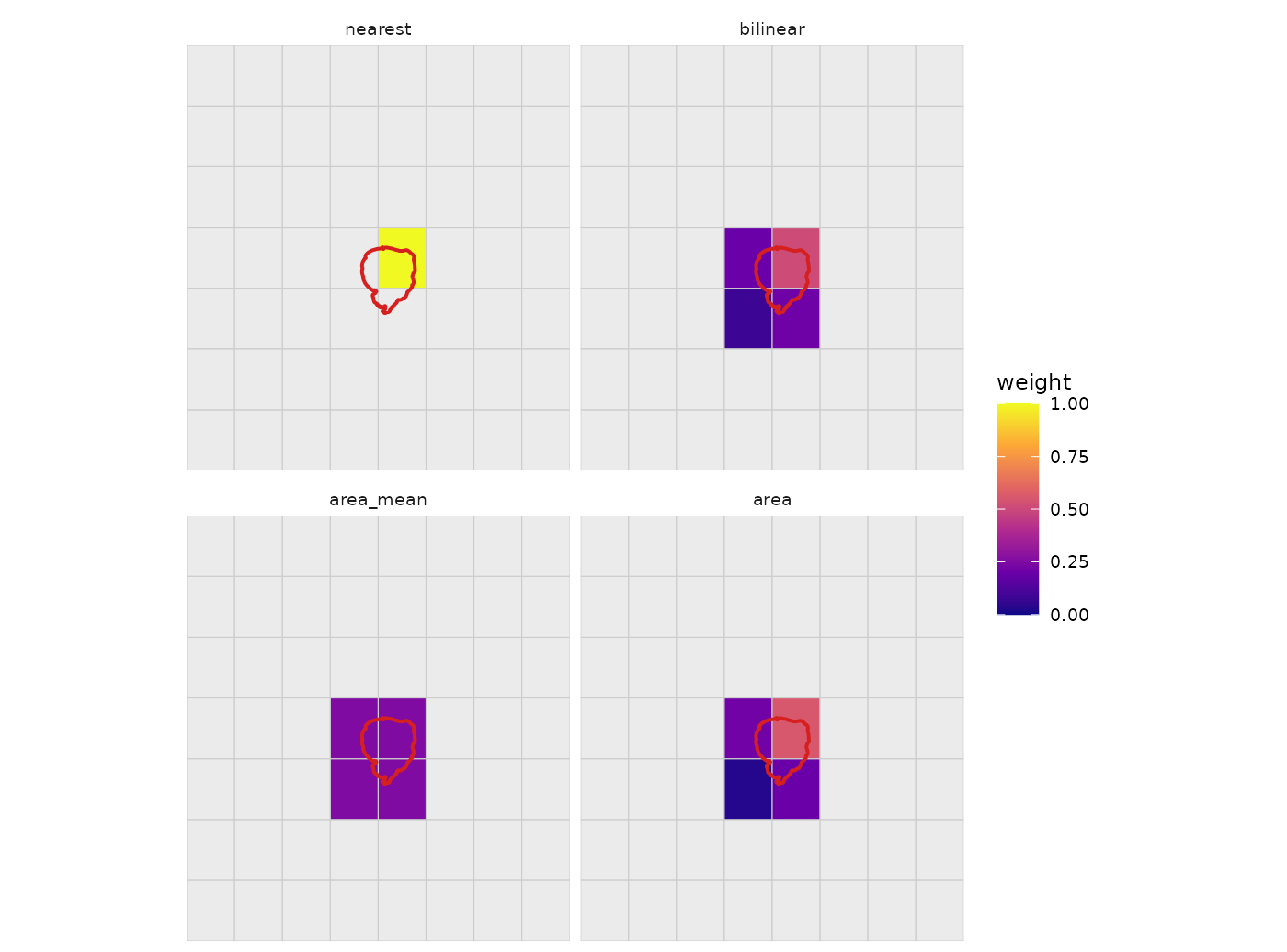
Figure 2. nearest takes the one cell
nearest the centroid; bilinear blends the four around it;
area_mean averages every cell the polygon overlaps with
equal weight; area weights those same cells by the share of
the polygon falling in each. Colour is the weight (summing to 1 in every
panel). Lake Rotorua covers an uneven 2×2 block, so area
and area_mean disagree — area is the honest
lake average.
Cells masked by ERA5-Land
ERA5-Land carries no data over the sea, and over some inland-water pixels. Masked cells are outlined dashed blue; the extractor drops them and rescales the surviving weights so they still sum to 1. Blanking the centre cell of the block:
centre <- attr(plot_extract_grid(gdir, geom = lake, method = "nearest"),
               "weights")
gdir_masked <- write_era5_land_grid(
  file.path(tempdir(), "era5_land_masked"),
  na_cells = list(c(centre$ix, centre$iy)))

plot_extract_grid(gdir_masked, geom = lake, method = "area")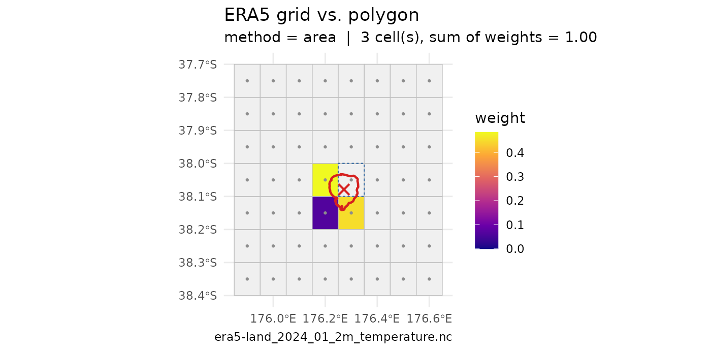
Figure 3. The centre cell masked (dashed blue) and
dropped from method = "area"; its weight is spread over the
three cells that remain. max_dist_km / the nearest-valid
fallback use the same mask, so a lake sitting entirely on masked pixels
still resolves to the closest cell that has data.
Other arguments
-
pad— grid cells of context drawn around the geometry (default3); raise it to see more of the surrounding grid. -
max_dist_km— for a"nearest"sample,plot_extract_grid()warns and still draws (with the distance in the subtitle) whereextract_era5_hourly_met()would stop with an error. -
area_crs— projected CRS the"area"intersection areas are computed in (default2193, NZTM 2000); use one suited to your region. -
engine = "base"— draw withsf::plot()instead of and return the gridsfinvisibly, for a dependency-free check. -
variables,pattern,years,months— passed straight to the file matcher, so the preview opens the same files the extraction will.
plot_extract_grid(gdir, lon = 178.0, lat = -38.0, method = "nearest",
                  max_dist_km = 50, pad = 2)
#> Warning: Nearest valid ERA5 cell is 114.0 km from (178.0000, -38.0000), beyond
#> max_dist_km = 50. Check lon/lat / the data region, or raise max_dist_km.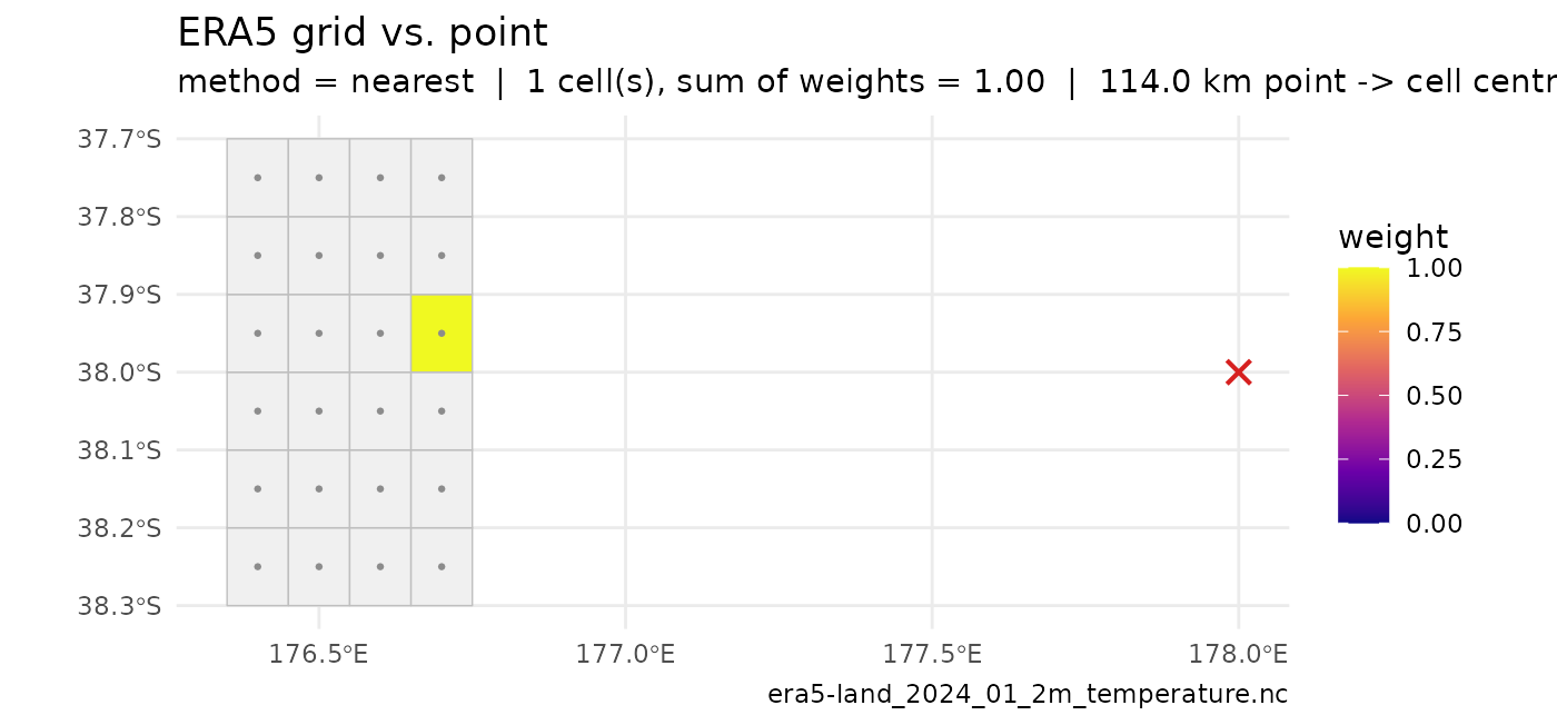
Figure 4. max_dist_km with a point ~110 km
east of the grid: plot_extract_grid() warns, picks the
nearest edge cell and draws it so the mistake is visible;
extract_era5_hourly_met(method = "nearest") would abort
with the same message.
extract_era5_lake_met() — the polygon wrapper
extract_era5_lake_met() is the same call with two
conveniences: method defaults to "area", and
optional id / name are stored on the result as
lake_id / lake_name attributes. The polygon
can be an sf / sfc object or a path to a
vector file (.gpkg, .shp,
.rds).
met <- extract_era5_lake_met(
  lake_poly,                     # or "gis/rotorua.gpkg"
  path    = "era5_netcdf",
  years   = 2023:2025,
  name    = "Rotorua",
  outfile = "rotorua_era5_hourly_met.csv")

## batch over a multi-lake layer
lakes <- sf::st_read("gis/lakes.gpkg")
mets  <- lapply(seq_len(nrow(lakes)), function(i)
  extract_era5_lake_met(lakes[i, ], path = "era5_netcdf", years = 2024,
                        id = lakes$id[i], name = lakes$name[i]))
The bundled rotorua_era5_hourly_met.csv.gz used
throughout the other vignettes is the output of exactly this call for
Lake Rotorua.
See also
-
vignette("download-era5")— getting the netCDF in the first place. -
vignette("met-data-frames")— theMET_*names, units and time-zone convention the extractor output follows. -
vignette("bias-correction-methods")— correcting the extracted series against local observations. -
?plot_extract_grid— the pre-extraction grid check shown above.