Rotorua QC Summary

Load libraries

library(dplyr)
library(tidyr)
library(readr)
library(lubridate)
library(ggplot2)
library(scattermore)
library(DT)
library(patchwork)

# Set timezone to NZST
withr::local_locale(c("LC_TIME" = "C"))
withr::local_timezone("Etc/GMT-12")

# Load functions
source("R/qc_funs.R")

1 Download data from GitHub

piggyback::pb_download(
  file = "rotorua_data_qc.zip",
  dest = ".",
  repo = "limnotrack/f_rotorua",
  tag = "v0.0.1"
)

# Unzip the file
unzip("rotorua_data_qc.zip")

2 Read data

path <- "rotorua_data_qc"

site <- read_csv("rotorua_data_qc/sites.csv", col_types = cols())
site_events <- read_csv("rotorua_data_qc/site_events.csv", col_types = cols())
site_devices <- read_csv("rotorua_data_qc/site_devices.csv", col_types = cols())
device_var <- read_csv("rotorua_data_qc/device_variable.csv", col_types = cols())
device_position <- read_csv("rotorua_data_qc/device_position.csv", 
                            col_types = cols())
sensor_reference <- read_csv("rotorua_data_qc/sensor_reference.csv",
                             col_types = cols())
sensor_calibrations <- read_csv("rotorua_data_qc/sensor_calibrations.csv", 
                                col_types = cols())
sensor_scaling <- read_csv("rotorua_data_qc/sensor_scaling.csv",
                           col_types = cols())
variable_ref <- read_csv("rotorua_data_qc/variables.csv", col_types = cols())
qc_filters <- read_csv("rotorua_data_qc/qc_filters.csv", col_types = cols())

data_wide <- read_csv("rotorua_data_qc/rotorua_qc.csv", col_types = cols())

Pivot the data to long format and map site devices.

data <- data_wide |> 
  pivot_longer(
    cols = matches("^(qc_value|qc_code|qc_flag)_"),
    names_to = c(".value", "var_ref_id"),
    names_pattern = "^(qc_value|qc_code|qc_flag)_(.+)$"
  )

# Map site devices to data
data <- data |> 
  map_data_to_devices(site_devices = site_devices,
                      device_var = device_var,
                      device_position = device_position,
                      variables = variable_ref
                      ) 
head(data)

# A tibble: 6 × 9
  site  device_id var_abbr var_ref_id label datetime            qc_value qc_code
  <chr> <chr>     <chr>    <chr>      <chr> <dttm>                 <dbl> <chr>  
1 f_Ro… sns_ZT_d… c_do     c_do_d100  Diss… 2007-07-13 14:45:00     11.0 QC 300 
2 f_Ro… sns_ZT_d… c_do     c_do_d100  Diss… 2007-07-13 15:00:00     11.3 QC 300 
3 f_Ro… sns_ZT_d… c_do     c_do_d100  Diss… 2007-07-13 15:15:00     11.3 QC 300 
4 f_Ro… sns_ZT_d… c_do     c_do_d100  Diss… 2007-07-13 15:30:00     11.1 QC 300 
5 f_Ro… sns_ZT_d… c_do     c_do_d100  Diss… 2007-07-13 15:45:00     11.2 QC 300 
6 f_Ro… sns_ZT_d… c_do     c_do_d100  Diss… 2007-07-13 16:00:00     11.2 QC 300 
# ℹ 1 more variable: qc_flag <chr>

3 Summarise by variable

Which variables are in the dataset?

Here is the list of variables in the dataset. The var_ref_id is the variable reference ID, which is used to identify the variable in the dataset. The var_abbr is the variable abbreviation, which is used to identify the variable in the metadata. The label is the variable label, which is used to identify the variable in the metadata. The reference is the reference value for the variable, it can be “d” (depth), “h” (height) or “e” elevation and the value_m is the value in meters.

data |> 
  select(var_ref_id) |> 
  distinct() |> 
  mutate(decode_var_ref(var_ref_id)) |>
  left_join(variable_ref, by = c("var_abbr" = "abbr")) |> 
  select(label, var_abbr, var_ref_id, reference, value_m) |> 
  datatable(rownames = FALSE,
            options = list(
              pageLength = 6,
              # dom = "t",
              columnDefs = list(list(className = 'dt-center', targets = "_all"))
            )
  ) 

Table 1

data |> 
  group_by(label) |> 
  summarise(
    min = min(qc_value, na.rm = TRUE),
    max = max(qc_value, na.rm = TRUE),
    median = median(qc_value, na.rm = TRUE),
    mean = mean(qc_value, na.rm = TRUE),
    sd = sd(qc_value, na.rm = TRUE),
    n = n(),
    na_pct = 100 * sum(is.na(qc_value)) / n(),
    qc_pct = 100 * sum(qc_code %in% c("QC 300", "QC 400",
                                      "QC 500", "QC 600")) / n(),
  ) |> 
  # Round everything to 1
  mutate(across(where(is.numeric), ~ round(.x, 1))) |> 
  DT::datatable()

4 Quality control

We used a set of quality control codes to assess the quality of the data. The codes are from the National Environmental Monitoring Standards (NEMS). The codes are as follows:

Table 2: Quality control codes used in the dataset.

5 Visualise each variable

The plots below show the A) time series of the data, B) the quality codes (QC) attributed to each data point, C) the device used to measure the data.

5.1 Temperature

plot_var_ts_qc(data = data, var_ref_id = c("t_wtr_d50", "t_wtr_d100",
                                           "t_wtr_d250", "t_wtr_d450",
                                           "t_wtr_d650", "t_wtr_d850",
                                           "t_wtr_d1050", "t_wtr_d1250",
                                           "t_wtr_d1450", "t_wtr_d1650", 
                                           "t_wtr_d1850", "t_wtr_d2000",
                                           "t_wtr_d2050"))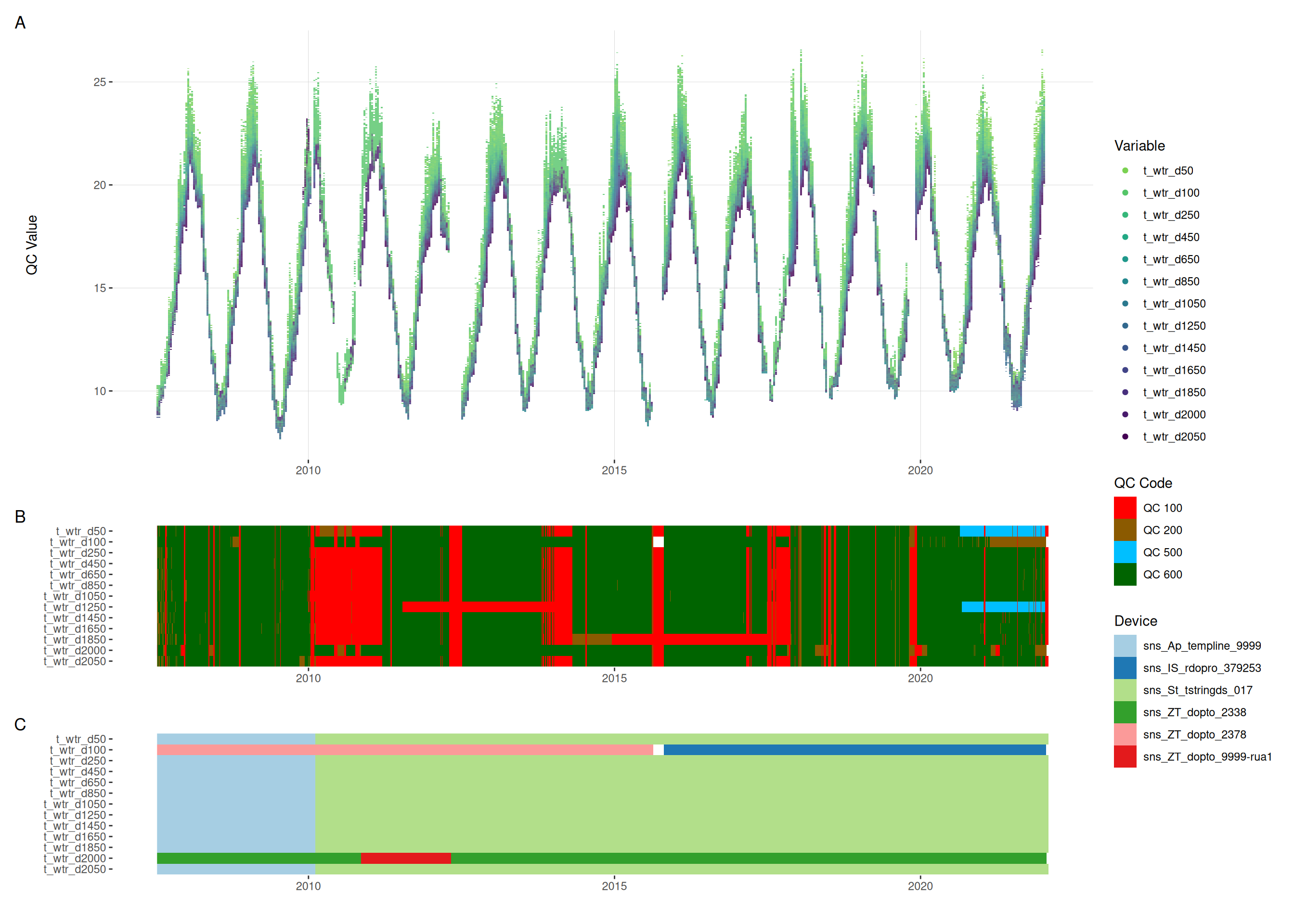

Figure 1: Temperature data at various depths quality control.

5.2 Oxygen saturation

plot_var_ts_qc(data = data, var_ref_id = c("c_do_sat_d100", "c_do_sat_d2000"))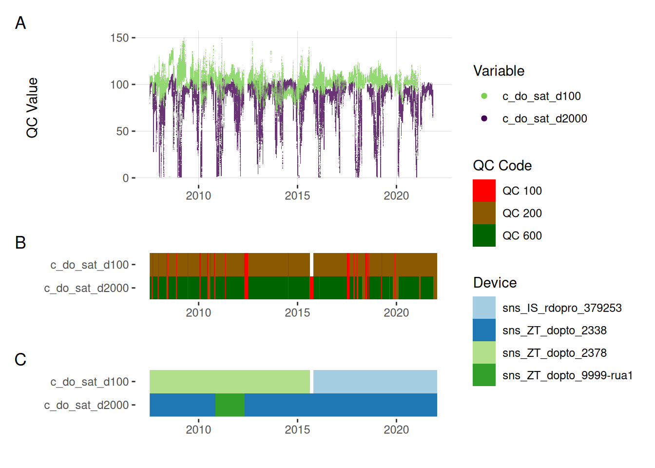

Figure 2: Oxygen saturation data at 1 and 10m depths quality control.

5.3 Oxygen concentration

plot_var_ts_qc(data = data, var_ref_id = c("c_do_d100", "c_do_d2000"))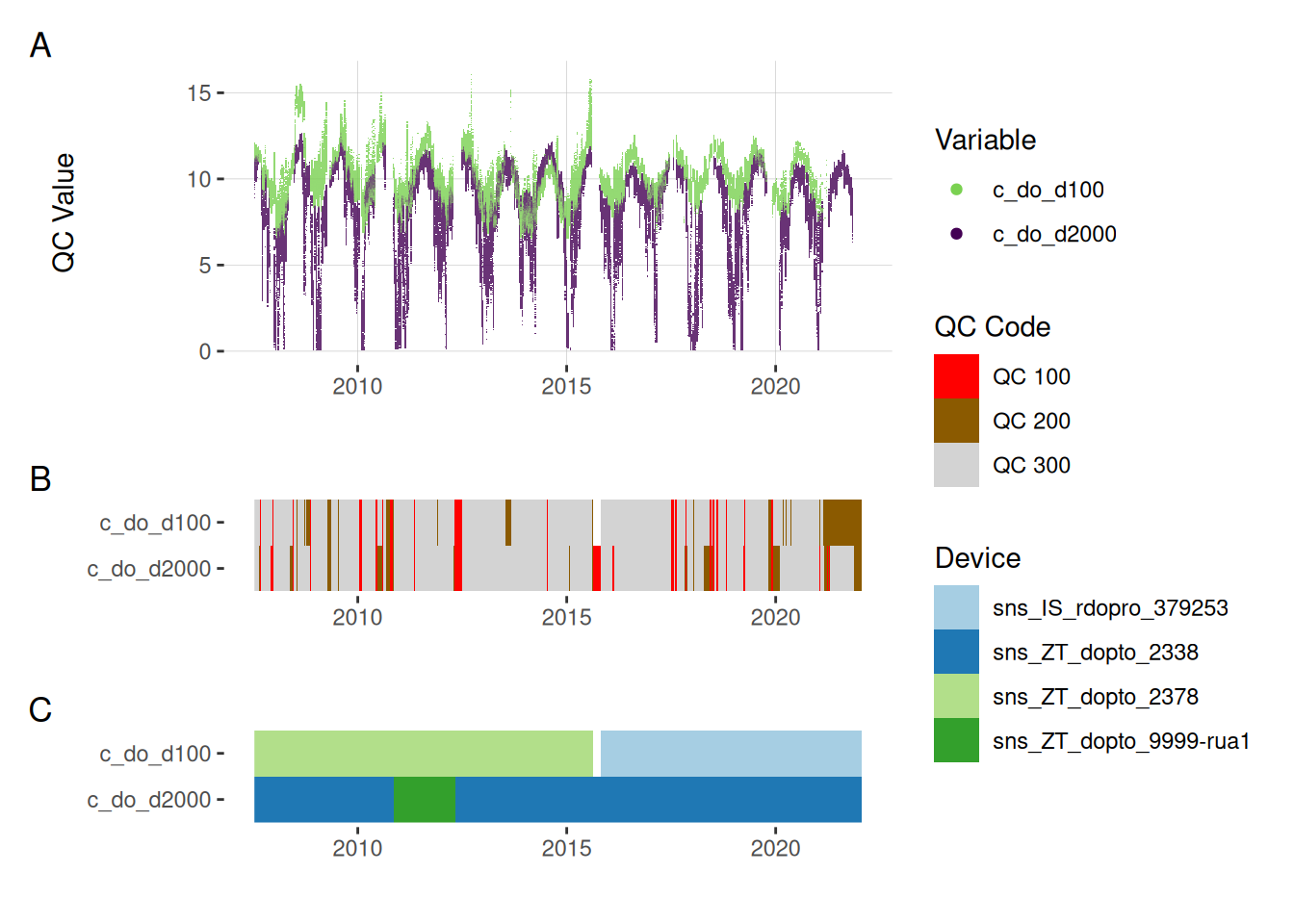

Figure 3: Oxygen data at 1 and 10m depths quality control.

5.4 Chlorophyll

plot_var_ts_qc(data = data, var_ref_id = c("f_chl_d100"))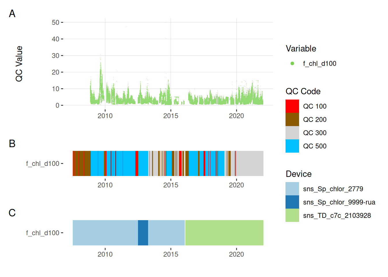

Figure 4: Chlorophyll data at 1.0m quality control.

5.5 Phycocyanin

plot_var_ts_qc(data = data, var_ref_id = c("f_phyc_d100"))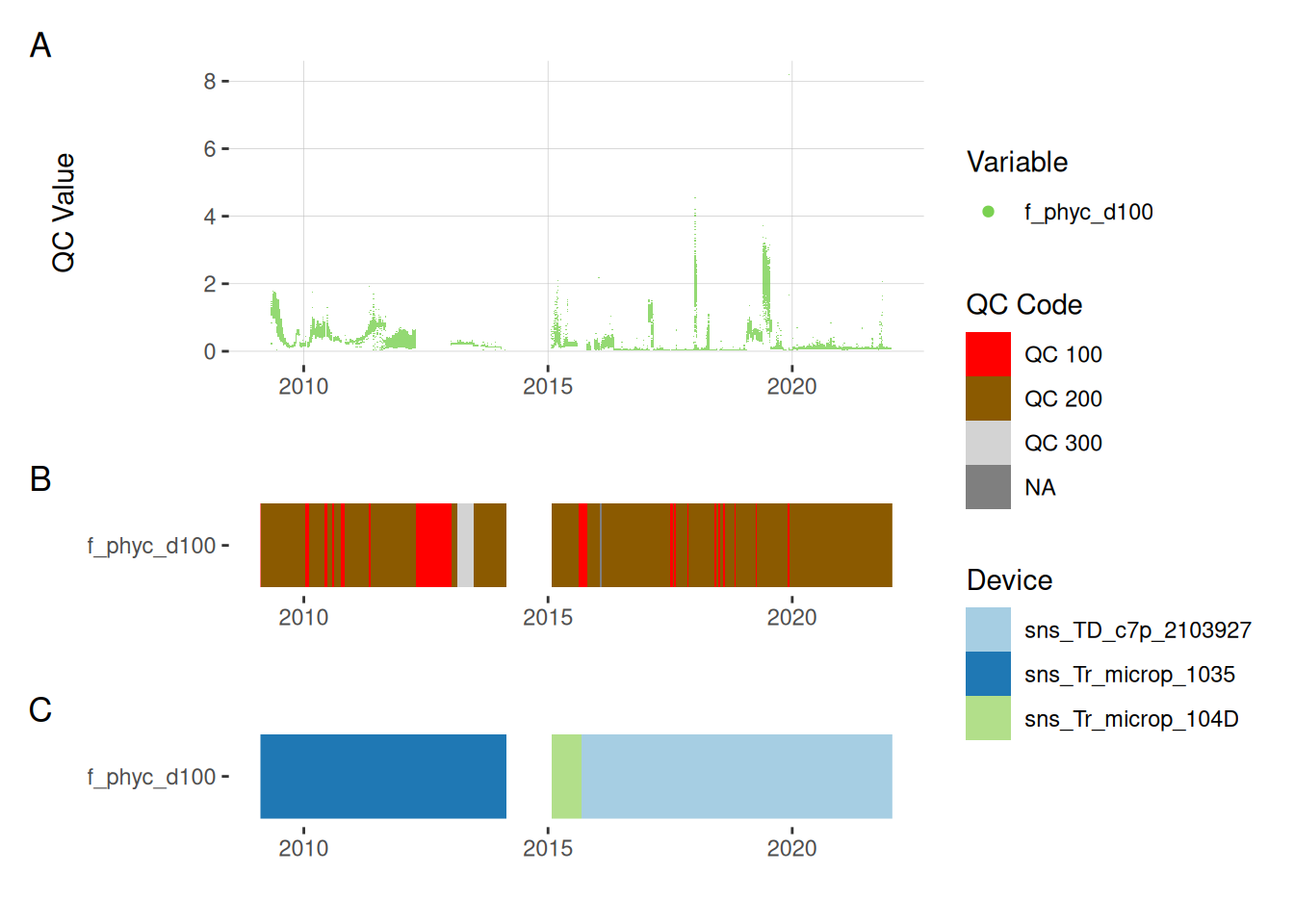

Figure 5: Phycocyanin data at 1.0m quality control.

5.6 pH

plot_var_ts_qc(data = data, var_ref_id = c("c_ph_d100"))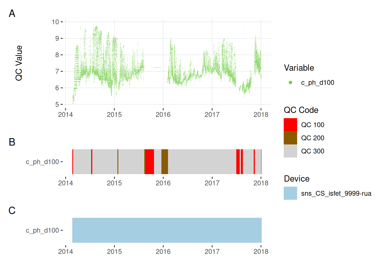

Figure 6: pH data at 1.0m quality control.

6 Download data

The data used in this analysis is available for download. The data is in CSV format and is zipped. The data is in the rotorua_data_qc.zip folder. The data can be downloaded either from GitHub or from the button below.

Download Data